Weighting and Its Consequences

Note

This is the fourth entry in a multi-part series of posts on weighting surveys. You can read the previous entries at the links below.

• Part 1: The Abstract
• Part 2: A Free Lunch
• Part 3: Binary Surprises

library(tidyverse)

In this series of posts thus far, I’ve explored how weighting survey responses affects (and, importantly, can reduce) the bias and variance of the population mean estimate for both continuous and discrete outcomes. While this is pedagogically interesting for both producers and consumers of individual poll results, I am personally more interested in how this affects models estimating public opinion from multiple polls. In this post, I’ll demonstrate that aggregators, forecasters, and researchers can improve the precision of parameter estimates by modeling each poll’s variance directly.

To get started, let’s consider a population with two variables that we can stratify by, with two classes within each strata, for a total of four groups in the population. For simplicity’s sake, we’ll assume that the groups are of equal size. We’ll be simulating pre-election poll responses as a binary choice between the democratic and republican candidate from this population and enforce the fact that group membership is highly correlated with candidate preference.

groups <- read_csv("data/groups.csv")
pollsters <- read_csv("data/pollsters.csv")
polls <- read_rds("data/polls.rds")

groups %>%
  select(strata_1, strata_2, group, group_mean) %>%
  knitr::kable()

strata_1	strata_2	group	group_mean
A	1	A1	0.97
A	2	A2	0.90
B	1	B1	0.10
B	2	B2	0.03

Let’s also simulate a set of pollsters who will be conducting these simulated polls. These pollsters will have different statistical biases¹ that we’ll want to incorporate as a part of the model. Further, each pollster will employ one of two possible weighting strategies: “single” or “cross.”

¹ As measured on the logit scale.

pollsters %>%
  select(pollster, strategy, bias) %>%
  knitr::kable()

pollster	strategy	bias
Pollster 1	cross	-0.0280238
Pollster 2	cross	-0.0115089
Pollster 3	cross	0.0779354
Pollster 4	cross	0.0035254
Pollster 5	cross	0.0064644
Pollster 6	cross	0.0857532
Pollster 7	cross	0.0230458
Pollster 8	cross	-0.0632531
Pollster 9	cross	-0.0343426
Pollster 10	cross	-0.0222831
Pollster 11	single	0.0612041
Pollster 12	single	0.0179907
Pollster 13	single	0.0200386
Pollster 14	single	0.0055341
Pollster 15	single	-0.0277921
Pollster 16	single	0.0893457
Pollster 17	single	0.0248925
Pollster 18	single	-0.0983309
Pollster 19	single	0.0350678
Pollster 20	single	-0.0236396

Pollsters that use the “cross” strategy will estimate the population mean by weighting on all variables (i.e., the cross of strata_1 and strata_2) whereas pollsters that use the “single” strategy will only weight responses by strata_2. Effectively, this means that pollsters using the “single” strategy will weight on variables that are not highly correlated with the outcome.

groups %>%
  group_by(strata_2) %>%
  summarise(strata_mean = mean(group_mean)) %>%
  knitr::kable()

strata_2	strata_mean
1	0.535
2	0.465

If we simulate a set of polls under these assumptions, however, we won’t have access to the underlying group response data. Instead, the dataset that will feed into the model will include topline information per poll. Here, pollsters are reporting the mean estimate for support for the democratic candidate along with the sample size and margin of error.

polls %>%
  slice_head(n = 10) %>%
  transmute(day = day,
            pollster = pollster,
            sample_size = map_int(data, ~sum(.x$K)),
            mean = mean,
            err = pmap_dbl(list(mean, sd), ~(qnorm(0.975, ..1, ..2) - ..1))) %>%
  mutate(across(c(mean, err), ~scales::label_percent(accuracy = 0.1)(.x)),
         err = paste0("+/-", err)) %>%
  knitr::kable()

day	pollster	sample_size	mean	err
1	Pollster 2	941	49.5%	+/-1.6%
1	Pollster 8	987	48.1%	+/-1.5%
1	Pollster 11	863	53.6%	+/-3.3%
2	Pollster 11	847	51.7%	+/-3.4%
2	Pollster 12	949	54.1%	+/-3.1%
2	Pollster 20	948	49.0%	+/-3.2%
3	Pollster 8	973	50.7%	+/-1.7%
3	Pollster 20	1048	48.1%	+/-3.1%
4	Pollster 10	933	49.4%	+/-1.7%
4	Pollster 19	1161	52.3%	+/-2.9%

How might we model the underlying support the democratic candidate given this data? A reasonable approach would be to follow the approach described in Drew Linzer’s 2013 paper, Dynamic Bayesian Forecasting of Presidential Elections in the States.² Here, the number of responses supporting the democratic candidate in each poll is estimated as round(mean * sample_size), after which a binomial likelihood is used to estimate the model. So our dataset prepped for modeling will look something like this:

² Notably, variations of this approach have been used used by Pierre Kemp in 2016, the Economist in 2020, and myself in 2024.

polls %>%
  slice_head(n = 10) %>%
  transmute(day = day,
            pollster = pollster,
            sample_size = map_int(data, ~sum(.x$K)),
            mean = mean,
            err = pmap_dbl(list(mean, sd), ~(qnorm(0.975, ..1, ..2) - ..1))) %>%
  mutate(err = scales::label_percent(accuracy = 0.1)(err),
         err = paste0("+/-", err),
         Y = round(mean * sample_size),
         K = sample_size,
         mean = scales::label_percent(accuracy = 0.1)(mean)) %>%
  knitr::kable()

day	pollster	sample_size	mean	err	Y	K
1	Pollster 2	941	49.5%	+/-1.6%	466	941
1	Pollster 8	987	48.1%	+/-1.5%	475	987
1	Pollster 11	863	53.6%	+/-3.3%	462	863
2	Pollster 11	847	51.7%	+/-3.4%	438	847
2	Pollster 12	949	54.1%	+/-3.1%	514	949
2	Pollster 20	948	49.0%	+/-3.2%	465	948
3	Pollster 8	973	50.7%	+/-1.7%	493	973
3	Pollster 20	1048	48.1%	+/-3.1%	504	1048
4	Pollster 10	933	49.4%	+/-1.7%	461	933
4	Pollster 19	1161	52.3%	+/-2.9%	608	1161

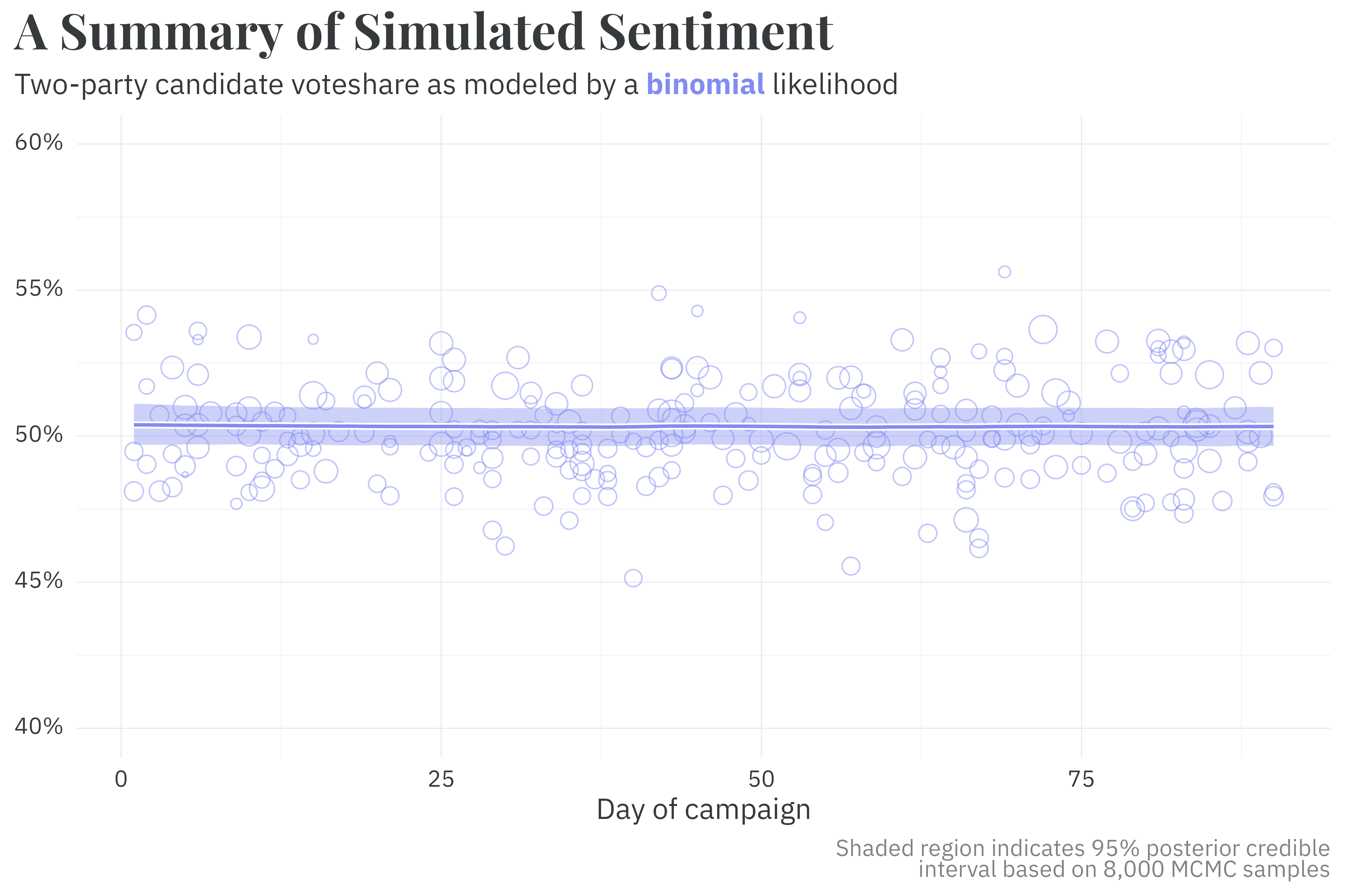
For a poll observed on day \(d\) conducted by pollster \(p\), I model the number of poll respondents supporting the democratic candidate, \(\text{Y}_{d,p}\), as binomially distributed given the poll’s sample size, \(\text{K}_{d,p}\), and the poll-specific probability of support, \(\theta_{d,p}\).

\[ \begin{align*} \text{Y}_{d,p} &\sim \text{Binomial}(\text{K}_{d,p}, \theta_{d,p}) \end{align*} \]

I model the latent support per poll with parameters measuring change in candidate support over time, \(\beta_d\),³ and parameters measuring the statistical bias per pollster, \(\beta_p\). \(\beta_p\) is modeled as hierarchically distributed with a standard distribution of \(\sigma_\beta\).

³ This is modeled as a gaussian random walk, but I’ve affixed this to be unchanging over time.

\[ \begin{align*} \text{logit}(\theta_{d,p}) &= \alpha + \beta_d + \beta_p \\ \beta_p &= \eta_p \sigma_\beta \end{align*} \]

The estimated true latent support is simply the daily fit excluding any pollster biases. I.e., \(\text{logit}(\theta_d) = \alpha + \beta_d\). The model samples efficiently and captures the latent trend well enough.

Similarly, the fitted model recovers the true parameters measuring pollster bias across pollsters using either weighting strategy.

This is all well and good, but can potentially be better! This approach discards some important information: the reported margin of error from each poll is ignored. The model implicitly infers a margin of error given the sample size. But as discussed in previous posts, weighting on variables highly correlated with the outcome can reduce the variance of the estimated mean! We can do better by modeling the variance of each poll directly, given each poll’s reported margin of error.

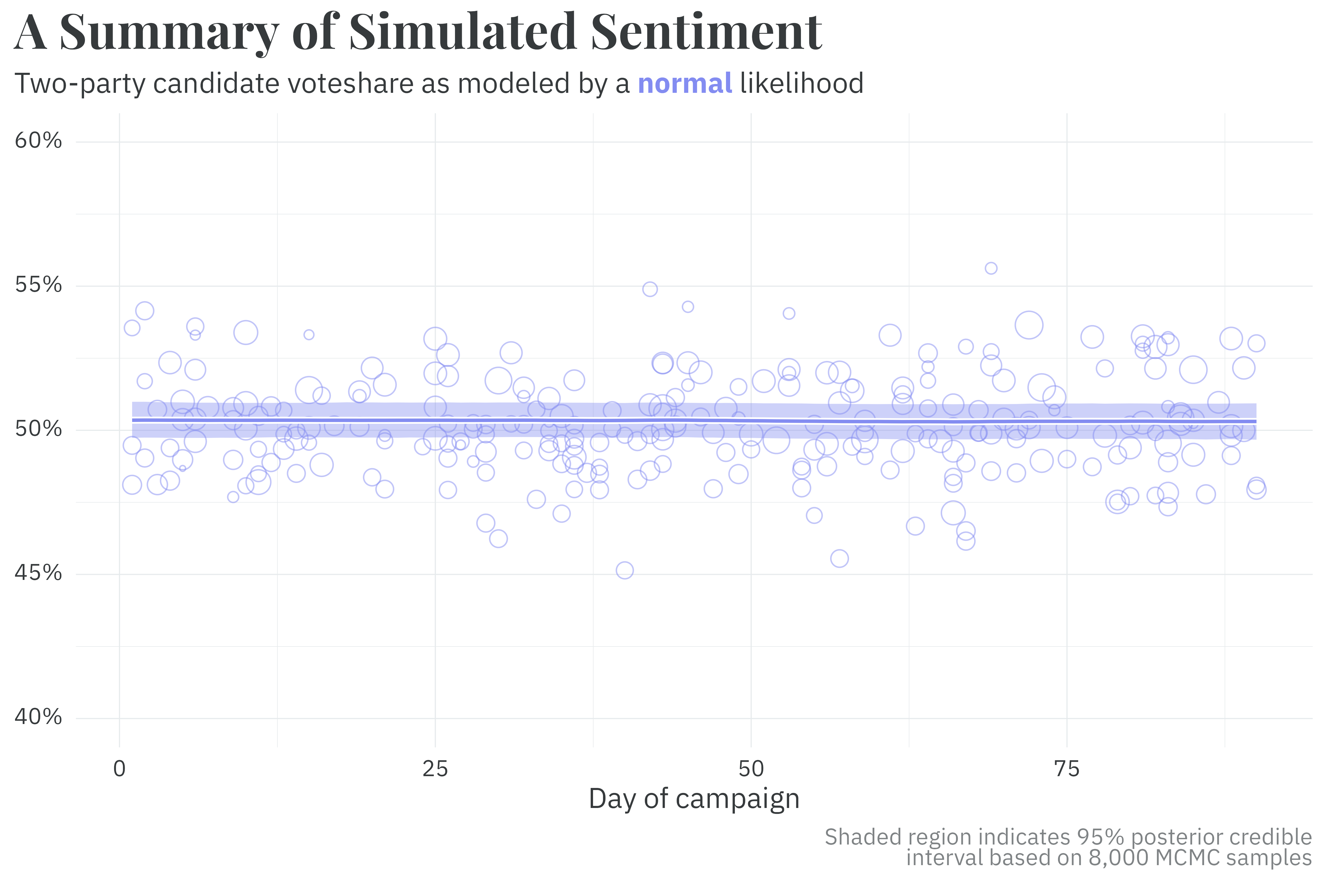
To do so, we only need to make a small change to the likelihood. Here, we redefine \(\text{Y}_{d,p}\) to be the observed mean of each poll and \(\sigma_{d,p}\) to be the standard deviation of each poll (inferred from the margin of error). We can then simply swap the binomial likelihood for a normal likelihood and leave the rest of the model the same.

\[ \text{Y}_{d,p} \sim \text{Normal}(\theta_{d,p}, \sigma_{d,p}) \]

Under this formulation, the model still samples efficiently⁴ and captures the latent trend well — the posterior estimates for \(\theta_d\) are close-to-unchanged from the binomial model.

⁴ In this particular case, it samples more efficiently.

The parameters measuring pollster bias, however, are more precise among pollsters who weight responses on variables highly correlated with the outcome, while still recovering the true parameters. The posterior bias parameters among pollsters who use the “single” weighting strategy have about the same level of precision as in the previous model.

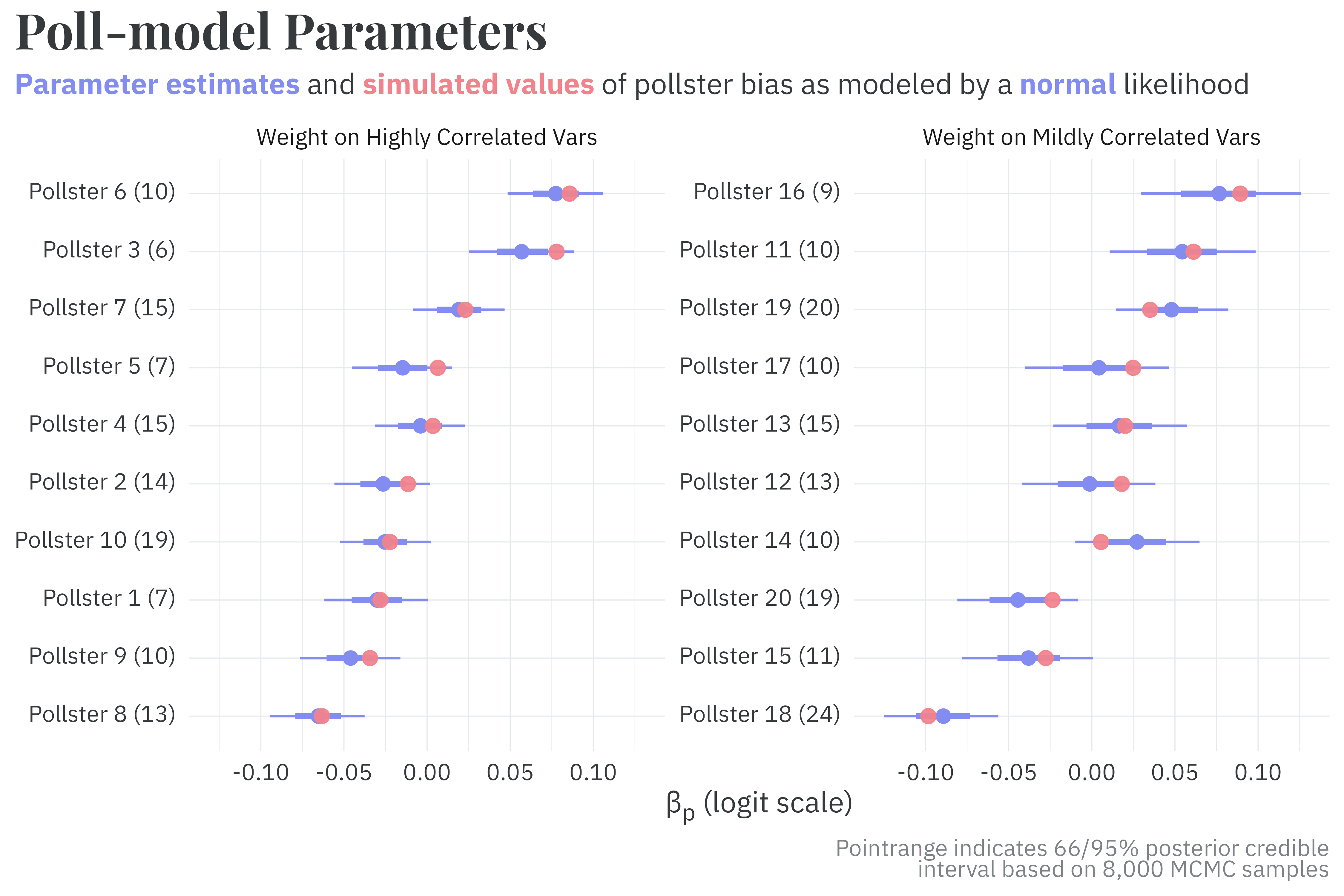
Other parameterizations, such as using the mean-variance formulation of the beta distribution for the likelihood, also see this benefit. Regardless of the specific likelihood used, the point here is that modeling the reported uncertainty in each poll, rather than using a binomial likelihood, can improve the precision of parameter estimates.