Weighting and Its Consequences

Note

This is the second entry in a multi-part series of posts on weighting surveys. You can read the first part here.

library(tidyverse)
library(ggdist)
library(ggblend)
library(riekelib)

pal <- c("#838cf1", "#f1838c", "#5a9282")

Methodological choices when conducting statistical analyses are all about balancing trade-offs — statisticians generally must choose to gain one benefit at the cost of another. The most prescient of these is the bias-variance trade-off but other examples include choosing to build a performant predictive model at the cost of a causal interpretation or choosing a parsimonious and explainable model at the cost of the improved accuracy that can accompany a more complex model.

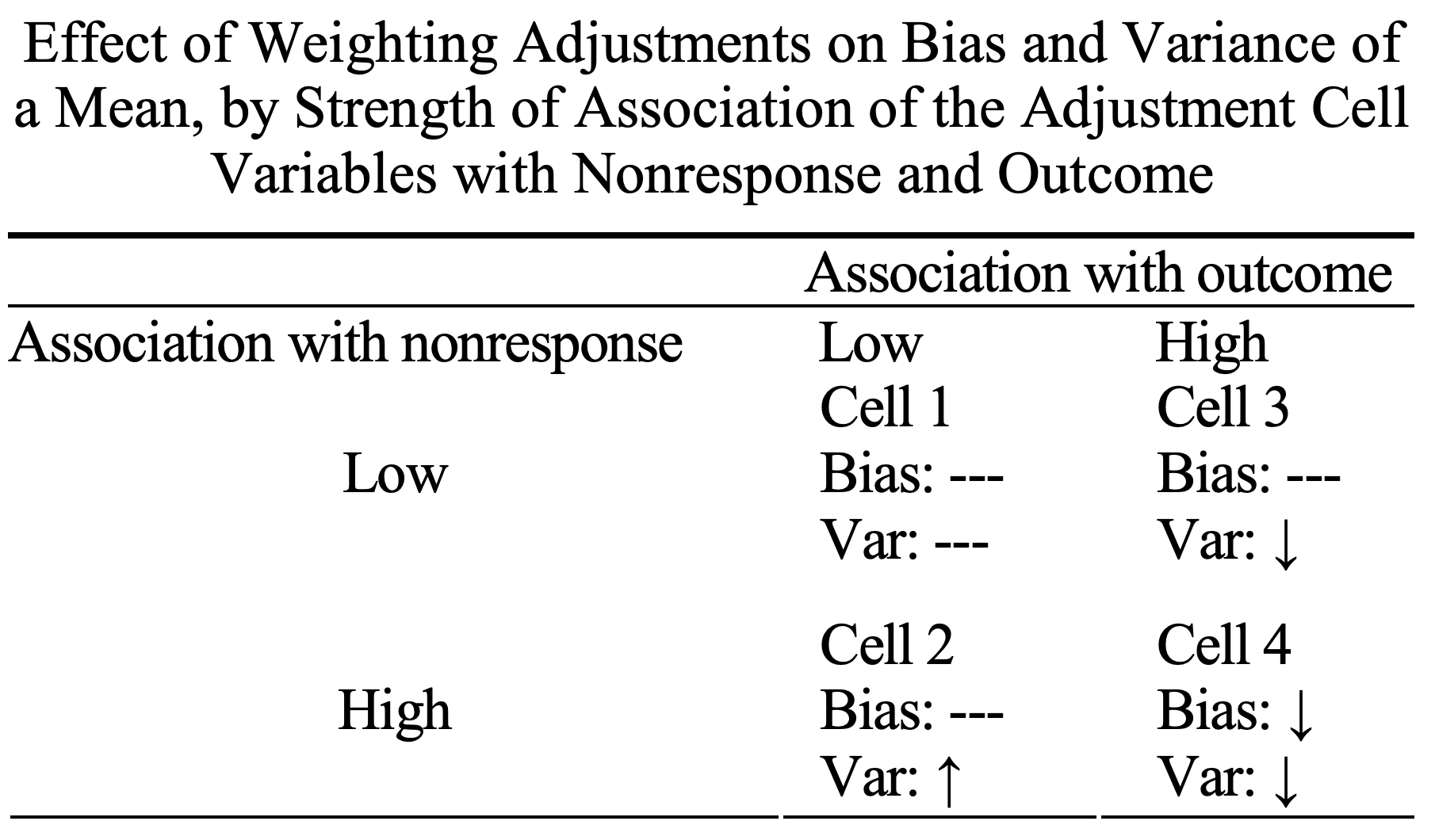
In some cases, however, a methodological choice is a free lunch — all benefit with no drawback. Drs. Roderick Little and Sonya Vartivarian highlight one such free lunch in the field of survey analysis in their 2005 paper, Does Weighting for Nonresponse Increase the Variance of Survey Means? As an excerpt from their abstract describes, weighting responses by subgroups can reduce both the bias and variance of the population mean estimate:

Nonresponse weighting is a common method for handling unit nonresponse in surveys. The method is aimed at reducing nonresponse bias, and it is often accompanied by an increase in variance. Hence, the efficacy of weighting adjustments is often seen as a bias-variance trade-off. This view is an oversimplification – nonresponse weighting can in fact lead to a reduction in variance as well as bias. A covariate for a weighting adjustment must have two characteristics to reduce nonresponse bias – it needs to be related to the probability of response, and it needs to be related to the survey outcome.¹

¹ Emphasis added.

The authors summarize the effect of weighting survey responses by subgroup membership in Table 1 of the paper. In plain English, they find that weighting:

• Has no effect on bias nor variance of the population mean estimate when subgroup membership is neither correlated with nonresponse nor the outcome (Cell 1);
• Has no effect on bias but increases the variance of the population mean estimate when subgroup membership is highly correlated with nonresponse but uncorrelated with the outcome (Cell 2);
• Has no effect on bias but decreases the variance of the population mean estimate when subgroup membership is uncorrelated with nonresponse but highly correlated with the outcome (Cell 3);
• Decreases both bias and variance of the population mean estimate when subgroup membership is correlated with both nonresponse and the outcome (Cell 4).

I’ll be honest — this feels like an unintuitive result! It feels like a decrease in bias should come at the cost of an increase in variance.² The best way to check my intuition, however, is through simulation.

² I am explicitly guilty of not understanding the effect of weighting on survey variance.

Here, I recreate the results of the paper using simulated survey responses for a continuous outcome. Let’s say we’re measuring respondents’ annual spend on some consumer goods category across four different regional subgroups and that we know the proportion of the population that belongs to each region.

# true underlying population/group characteristics
groups <-
  tibble(group = LETTERS[1:4],
         group_mean = c(400, 800, 700, 600),
         population = c(0.6, 0.2, 0.1, 0.1),
         p_respond = c(0.1, 0.05, 0.03, 0.01)) %>%
  mutate(p_sampled = population * p_respond,
         p_sampled = p_sampled/sum(p_sampled))

groups %>%
  select(group, population) %>%
  mutate(population = scales::label_percent()(population)) %>%
  knitr::kable()

group	population
A	60%
B	20%
C	10%
D	10%

I use a simplified inverse-probability weighting strategy ensure that the weighted survey sample has the same proportion of each subgroup as the population. Here, \(w_g\) is the weight applied to each respondent in subgroup \(g\), \(P_g\) is the proportion of subgroup \(g\) in the population, and \(N_g\) is the number of survey respondents in subgroup \(g\).

\[ w_g = \frac{P_g}{\left(\frac{N_g}{\sum_g N_g}\right)} \]

Under this setup, I simulate the results of 20,000 surveys — 5,000 for each of the four combinations of subgroup correlation with nonresponse and the outcome described by Little and Vartivarian. For each simulated survey, I compute the unweighted and weighted population mean estimates. I find that the distribution of the weighted and unweighted population mean estimates exhibit the behavior described in Little and Vartivarian’s paper.

# true mean among population
true_mean <-
  groups %>%
  summarise(true_mean = sum(group_mean * population)) %>%
  pull(true_mean)

# simulation parameters
n_sims <- 5000
sample_size <- 700
sigma <- 50

# plot! ------------------------------------------------------------------------

# setup simulation conditions
crossing(poll = 1:n_sims,
         differential_response = c(TRUE, FALSE),
         group_correlation = c(TRUE, FALSE),
         group = groups$group) %>%
  left_join(groups) %>%
  mutate(p_sampled = if_else(differential_response, p_sampled, population),
         group_mean = if_else(group_correlation, group_mean, true_mean)) %>%
  
  # simulate responses
  nest(data = -c(poll, differential_response, group_correlation)) %>%
  mutate(K = map(data, ~rmultinom(1, sample_size, .x$p_sampled)[,1])) %>%
  unnest(c(data, K)) %>%
  uncount(K) %>%
  bind_cols(Y = rnorm(nrow(.), .$group_mean, sigma)) %>%
  
  # summarize weighted/unweighted mean per simulation
  group_by(poll,
           group,
           differential_response,
           group_correlation) %>%
  mutate(n_group = n()) %>%
  group_by(poll,
           differential_response,
           group_correlation) %>%
  mutate(n_total = n(),
         observed = n_group/n_total,
         weight = population/observed) %>%
  summarise(weighted = sum(Y * weight)/sum(weight),
            unweighted = mean(Y)) %>%
  ungroup() %>%
  
  # prep for plotting
  pivot_longer(ends_with("weighted"),
               names_to = "method",
               values_to = "p") %>%
  mutate(case = case_when(differential_response & group_correlation ~ "Cell 4: Bias ↓ Variance ↓",
                          !differential_response & group_correlation ~ "Cell 3: Bias -- Variance ↓",
                          differential_response & !group_correlation ~ "Cell 2: Bias -- Variance ↑",
                          !differential_response & !group_correlation ~ "Cell 1: Bias -- Variance --")) %>%
  
  # plot!
  ggplot(aes(x = case,
             y = p,
             color = method,
             fill = method)) + 
  stat_histinterval(slab_alpha = 0.75) %>% partition(vars(method)) %>% blend("darken") +
  geom_hline(yintercept = true_mean,
             linetype = "dotted",
             color = "gray40") +
  scale_color_manual(values = rev(pal[1:2])) + 
  scale_fill_manual(values = rev(pal[1:2])) + 
  coord_flip() + 
  theme_rieke() + 
  theme(legend.position = "bottom") + 
  labs(title = "**Effect of weighting on estimates of the population mean**",
       subtitle = paste("Weighting on subgroups **decreases bias** and **decreases variance** when group",
                        "membership is highly correlated with response rate and preference in **continuous outcomes**",
                        sep = "<br>"),
       x = NULL,
       y = NULL,
       caption = paste("Distribution of weighted and unweighted population means for 5,000 simulated surveys",
                       "Dashed line indicates simulated true population mean",
                       sep = "<br>"))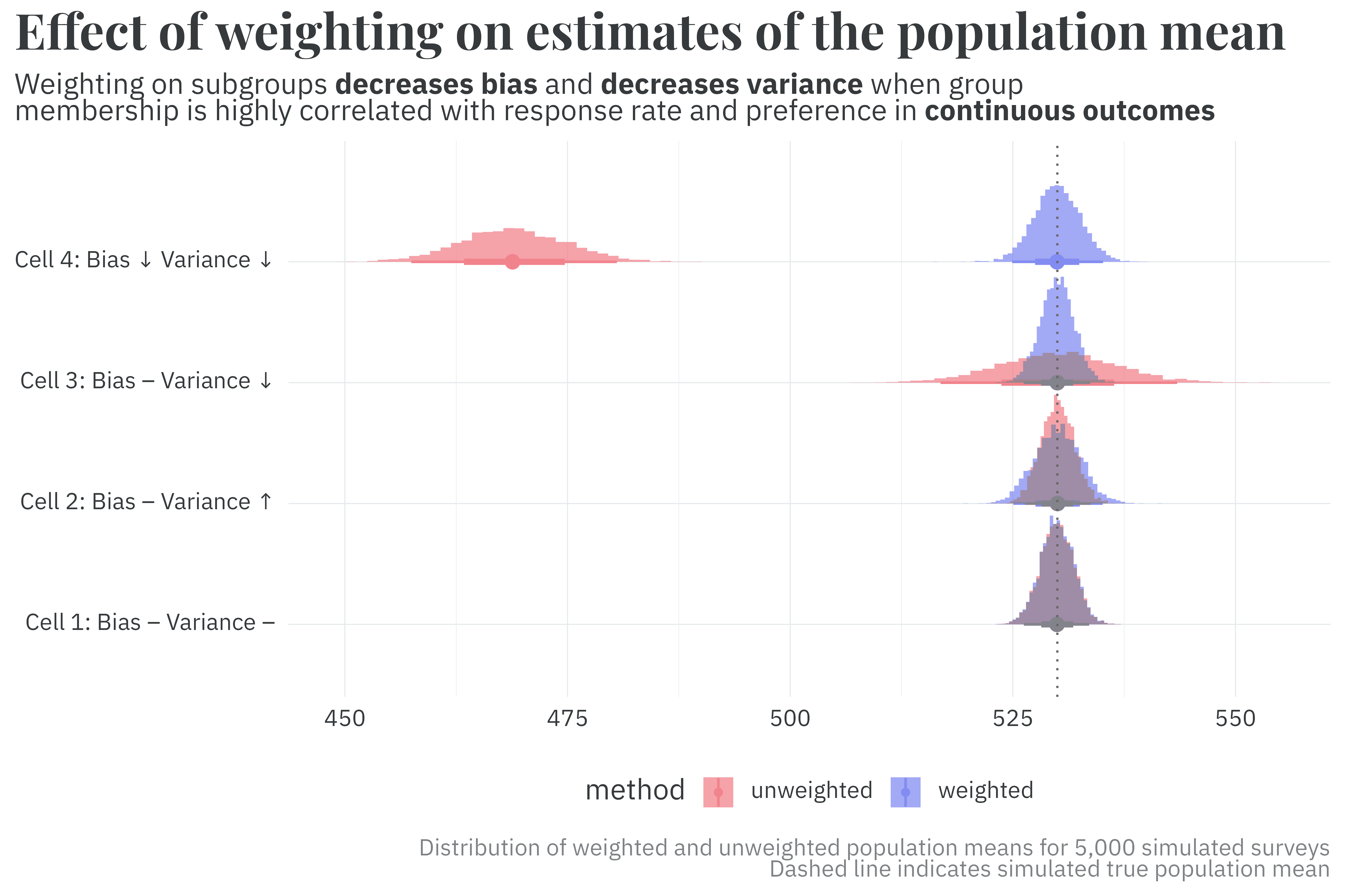

Great! Despite its seemingly unintuitive nature, simulating survey analyses confirms the results of the paper. A slight wrinkle, however — I first was introduced to this paper in the context of pre-election polling, where the outcome is discrete (a choice among a set of potential candidates). Here (and in Little and Vartivarian’s original paper), the effect of weighting given different combinations of correlation with nonresponse and the outcome is demonstrated using a continuous outcome. In the next post in this series, I’ll explore the effect weighting has on bias and variance given a discrete outcome.