Weighting and Its Consequences

Note

This is the third entry in a multi-part series of posts on weighting surveys. You can read the previous entries at the links below.

• Part 1: The Abstract
• Part 2: A Free Lunch

library(tidyverse)
library(ggdist)
library(ggblend)
library(riekelib)

pal <- c("#838cf1", "#f1838c", "#5a9282")

In the previous entry of this series on survey weighting, I recreated the results of Little and Vartivarian’s 2005 paper, Does Weighting for Nonresponse Increase the Variance of Survey Means? The paper (and my recreation) demonstrate that weighting survey responses can reduce both the bias and variance in the estimate of the population mean when the weighting variables are highly correlated with both the outcome and nonresponse.

These results were demonstrated using a continuous variable as the outcome. In many cases, however, surveys are designed to measure the population’s preference from a discrete set of choices.¹ How do Little and Vartivarian’s results hold up in surveys with discrete outcomes?

¹ Of particular interest to me (and regular readers here): political horse-race and issue polls all fall handily into this category.

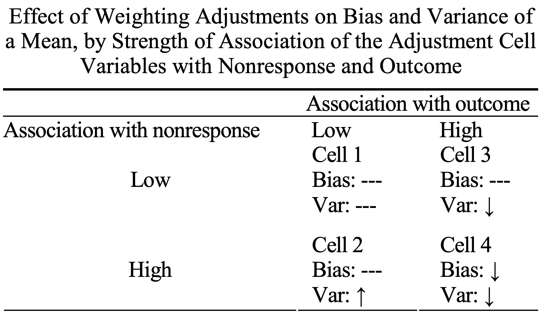
To answer this question, I once again turn to simulation. Consider two groups (A and B) of equal population answering a survey with a binary outcome. Much like the previous entry, we’ll set up four simulation sets that correspond to each of the cases in Little and Vartivarian’s paper:

• Case 1: Group membership is uncorrelated with both nonresponse and the outcome;
• Case 2: Group membership is uncorrelated with nonresponse but correlated with the outcome;
• Case 3: Group membership is correlated with nonresponse but uncorrelated with the outcome;
• Case 4: Group membership is correlated with both nonresponse and the outcome.

When group membership is correlated with the outcome, I set group A’s support at 3% and group B’s support to 97%. When correlated with nonresponse, I set group A’s probability of response to 5% and group B’s to 7%. Under these conditions, I simulate the results of 5,000 surveys per case and compare the unweighted and weighted² estimates to see the effect of weighting on bias and variance. In this particular set of binomial cases, weighting doesn’t quite display the same behavior observed in the continuous outcome case.

² I use the same simple inverse probability weighting method described in the previous post in this series.

# true underlying population/group characteristics
groups <-
  tibble(group = LETTERS[1:2],
         group_mean = c(0.03, 0.97),
         population = c(0.5, 0.5),
         p_respond = c(0.05, 0.07)) %>%
  mutate(p_sampled = population * p_respond,
         p_sampled = p_sampled/sum(p_sampled))

# true mean among population
true_mean <-
  groups %>%
  summarise(true_mean = sum(group_mean * population)) %>%
  pull(true_mean)

# simulation parameters
n_sims <- 5000
sample_size <- 700

# plot! ------------------------------------------------------------------------

# setup simulation conditions
crossing(poll = 1:n_sims,
         differential_response = c(TRUE, FALSE),
         group_correlation = c(TRUE, FALSE),
         group = groups$group) %>%
  left_join(groups) %>%
  mutate(p_sampled = if_else(differential_response, p_sampled, population),
         group_mean = if_else(group_correlation, group_mean, true_mean)) %>%
  
  # simulate responses
  nest(data = -c(poll, differential_response, group_correlation)) %>%
  mutate(K = map(data, ~rmultinom(1, sample_size, .x$p_sampled)[,1])) %>%
  unnest(c(data, K)) %>%
  bind_cols(Y = rbinom(nrow(.), .$K, .$group_mean)) %>%
  
  # summarize weighted/unweighted mean per simulation
  group_by(poll,
           differential_response,
           group_correlation) %>%
  mutate(n_total = sum(K),
         observed = K/n_total,
         weight = population/observed) %>%
  summarise(weighted = sum(Y * weight)/sum(K * weight),
            unweighted = sum(Y)/sum(K)) %>%
  ungroup() %>%
  
  # prep for plotting
  pivot_longer(ends_with("weighted"),
               names_to = "method",
               values_to = "p") %>%
  mutate(case = case_when(differential_response & group_correlation ~ "Cell 4: Bias ↓ Variance ↓",
                          !differential_response & group_correlation ~ "Cell 3: Bias -- Variance ↓",
                          differential_response & !group_correlation ~ "Cell 2: Bias -- Variance ↑",
                          !differential_response & !group_correlation ~ "Cell 1: Bias -- Variance --")) %>%
  
  # plot!
  ggplot(aes(x = case,
             y = p,
             color = method,
             fill = method)) + 
  stat_histinterval(slab_alpha = 0.75,
                    breaks = seq(from = 0.4, to = 0.7, by = 0.003125)) %>% partition(vars(method)) %>% blend("darken") +
  geom_hline(yintercept = true_mean,
             linetype = "dotted",
             color = "gray40") +
  scale_color_manual(values = rev(pal[1:2])) + 
  scale_fill_manual(values = rev(pal[1:2])) + 
  scale_y_percent() +
  coord_flip() + 
  theme_rieke() + 
  theme(legend.position = "bottom") + 
  labs(title = "**Effect of weighting on estimates of the population mean**",
       subtitle = paste("Weighting on subgroups **decreases biase** and **decreases variance** when group",
                        "membership is highly correlated with response rate and preference in **binary outcomes**",
                        sep = "<br>"),
       x = NULL,
       y = NULL,
       caption = paste("Distribution of weighted and unweighted population means for 5,000 simulated surveys",
                       "Dashed line indicates simulated true population mean",
                       sep = "<br>"))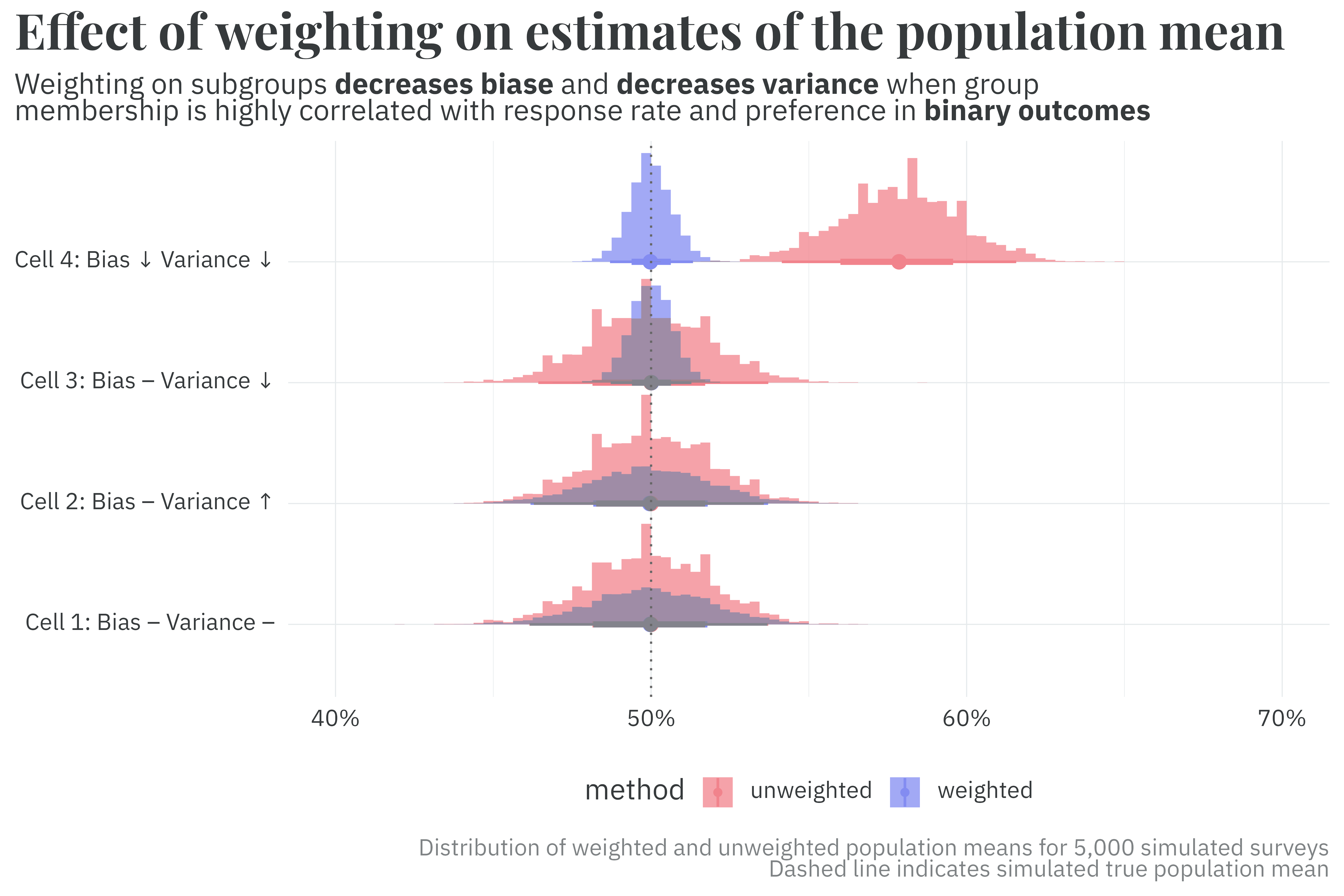

In cases 1 and 2, where group membership is uncorrelated with the outcome, we don’t see the same effects on variance as we did in the continuous case. In cases 3 and 4, we do, but only because I cranked up the group correlation with the outcome to an incredible degree. It appears that binomial outcomes require much more dramatic group differences than continuous outcomes in order to simultaneously decrease both bias and variance with survey weighting.

To explore when weighting benefits variance, I set up another set of simulations that vary the group correlation with both nonresponse and the outcome.³ By plotting the estimated standard error from 5,000 simulated surveys per combination of group correlation with nonresponse and the outcome, I find that:

³ In the plots below, support among group B is given as 1 - group_A_support.

• Any amount of group correlation with the outcome decreases the variance of the weighted population estimate relative to the unweighted estimate when group membership is uncorrelated with nonresponse;
• As group correlation with nonresponse increases, group correlation with the outcome must also increase dramatically in order to see a decrease in the variance of the population mean estimate. If groups are “not correlated enough” with the outcome, then weighting increases the variance of the population mean estimate.

# true underlying population/group characteristics
groups <-
  tibble(group = LETTERS[1:2],
         population = c(0.5, 0.5))

# simulation parameters
n_sims <- 5000
sample_size <- 700

# simulate responses -----------------------------------------------------------

sims <- 
  
  # simulate different levels of subgroup correlation with the outcome
  crossing(sim = 1:n_sims,
         beta = seq(from = 0.03, to = 0.97, by = 0.01),
         groups) %>%
  
  # simulate different levels of subgroup correlation with nonresponse
  nest(data = -c(sim, group, population)) %>%
  nest(data = -sim) %>%
  crossing(tibble(case = 1:4,
                  p_respond = list(c(0.05, 0.05), c(0.07, 0.03), c(0.08, 0.02), c(0.09, 0.01)))) %>%
  unnest(c(data, p_respond)) %>%
  unnest(data) %>%
  group_by(sim, beta, case) %>%
  mutate(p_sampled = population * p_respond,
         p_sampled = p_sampled/sum(p_sampled)) %>%
  ungroup() %>%
  
  # simulate survey collection / response
  mutate(p_support = if_else(group == "A", beta, 1 - beta)) %>%
  nest(data = -c(sim, beta, case)) %>%
  mutate(K = map(data, ~rmultinom(1, sample_size, .$p_sampled)[,1])) %>%
  unnest(c(data, K)) %>%
  bind_cols(Y = rbinom(nrow(.), .$K, .$p_support)) %>%
  
  # compute weighted/unweighted results per survey
  group_by(sim, beta, case) %>%
  mutate(n_total = sum(K),
         observed = K/n_total,
         weight = population/observed) %>%
  summarise(weighted = sum(Y * weight)/sum(K * weight),
            unweighted = sum(Y)/sum(K)) %>%
  ungroup() %>%
  
  # summarise mean/sd for each condition of case, p_support, and p_respond
  pivot_longer(ends_with("weighted"),
               names_to = "method",
               values_to = "p") %>%
  group_by(beta, method, case) %>%
  summarise(mean = mean(p),
            sd = sd(p)) %>%
  ungroup()
  
# plot! ------------------------------------------------------------------------

sims %>%
  mutate(case = case_match(case,
                           1 ~ "Response Rates: 5/5%",
                           2 ~ "Response Rates: 7/3%",
                           3 ~ "Response Rates: 8/2%",
                           4 ~ "Response Rates: 9/1%")) %>%
  ggplot(aes(x = beta,
             y = sd,
             color = method)) + 
  geom_point() +
  scale_color_manual(values = rev(pal[1:2])) + 
  facet_wrap(~case, scales = "free_y") + 
  theme_rieke() +
  theme(legend.position = "none") + 
  labs(title = "**Effect of weighting on SE of the mean**",
       subtitle = glue::glue("In binary outcomes, **",
                             color_text("weighting", pal[1]),
                             "** can reduce the SE relative to the **",
                             color_text("unweighted", pal[2]),
                             "** mean,<br>",
                             "depending on the relative proportion of nonresponse among subgroups"),
       x = "Subgroup A probability of support",
       y = "SE",
       caption = paste("SE estimated from 5,000 simulated surveys of 700 respondents",
                       "for each level of support among subgroup A",
                       sep = "<br>"))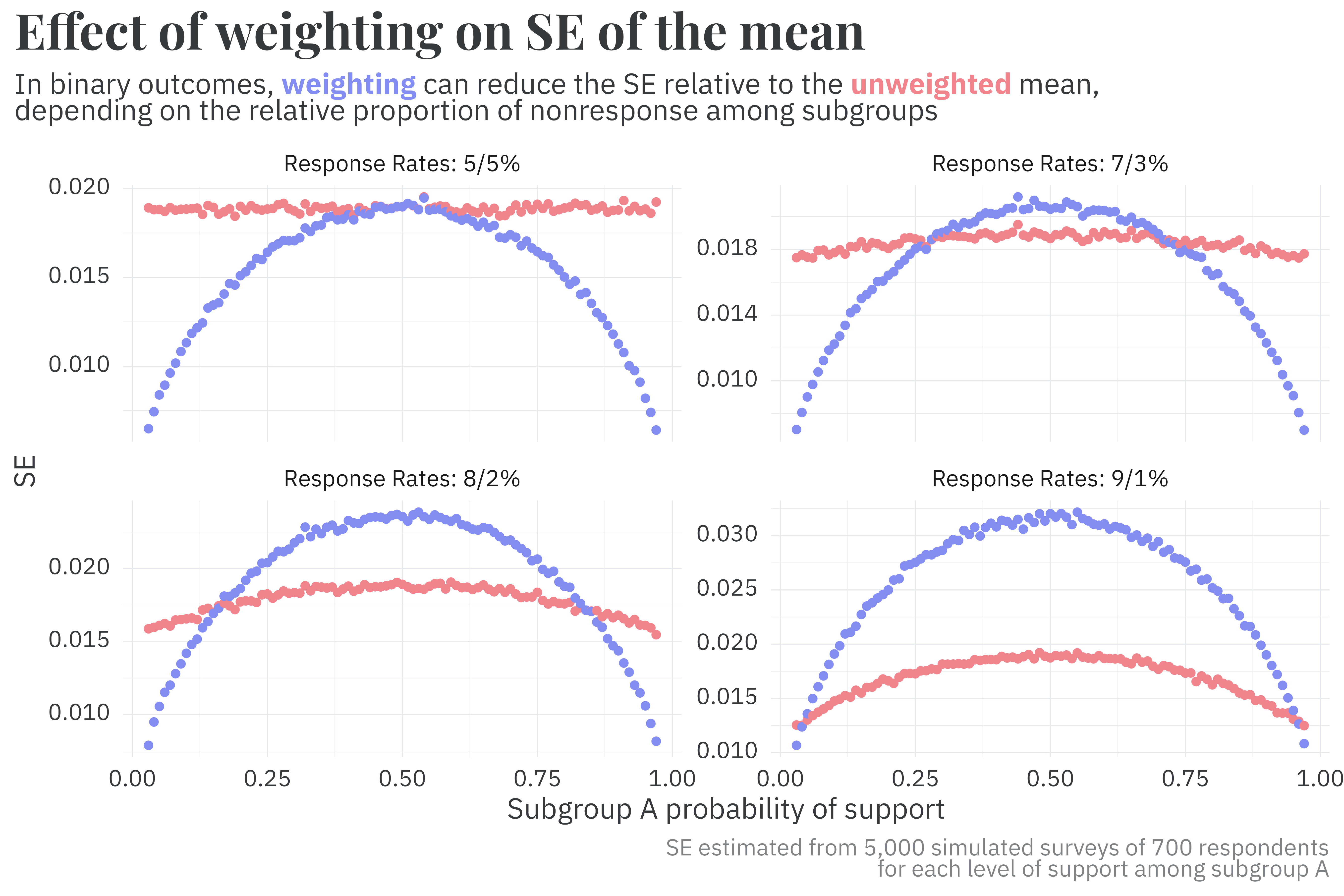

These findings are essentially in agreement with Little and Vartivarian’s paper, but offer some more detail about when a covariate is “correlated enough” with the outcome to decrease the variance in the estimate of the weighted mean. In short, the summary provided in Table 1 of Little and Vartivarian’s paper holds true, but what is considered “highly correlated” with the outcome is highly dependent on the level of differential nonresponse among subgroups. In particular, it appears that the benefit of weighting on variance requires surprisingly high degrees of correlation with binary outcomes.⁴

⁴ There’s a suspiciously parabola-like shape in the previous plot that implies a closed-form equation. I’ve gone down the rabbit hole of trying to find a nice and tidy general equation, but having seen that hell, I’m happy to settle for the results of simulation.

These findings are of interest for survey practitioners and analysts with access to the raw survey responses. I’m often more interested, however, in aggregating the results of political polls. In the next post in this series, I’ll demonstrate how aggregators/forecasters can incorporate the effects of weighting as a part of their models to decrease the variance in parameter estimates measuring statistical bias.