Free lunch at the vectorization table

Reparameterizing multinomial models for better computational efficiency
bayes
stan
rstats
Author

Mark Rieke

Published

April 26, 2023

I tend to find myself modeling categorical questions with many possible options. Questions on patient surveys have multiple options to choose from and there can be many possible candidates listed on an election poll. If modeling in Stan, the multinomial sampling statement is a natural tool to reach towards first. Multinomial models in Stan, however, cannot be vectorized1, so they can be very slow in comparison with other models. This can be pretty frustrating! And throwing more computational resources at the problem can help, but (from my experience), only marginally.

  • 1 Or, if they can, I am wholly unaware

  • Andrew Gelman, Bayesian benefactor that he is, has quite a few thoughts on how to address modeling issues. My favorite and most oft cited of which is the folk theorem of statistical computing, which states that computational issues are more often than not statistical issues in disguise and the solution is usually statistical, rather than computational.2 Perhaps unsurprisingly, this advice rings true in this scenario — this computational conundrum has a particularly satisfying statistical solution. With some (in hindsight, pretty simple) mathematical wizardry, we can rewrite a multinomial as a series of Poisson sampling statements.3 In this case, we’re truly getting a free lunch — this reparameterization provides the same inference as the original parameterization at a far quicker pace!

  • 2 Andrew Gelman et. al., “Bayesian workflow,” (November 2020), https://doi.org/10.48550/arXiv.2011.01808.

  • 3 Richard McElreath. Statistical Rethinking: A Bayesian Course with Examples in R and Stan (Boca Raton, FL: Chapman & Hall/CRC, 2020), 363-365.

  • To see this in action, let’s simulate some data and fit a few models. The code block below generates a multinomial response matrix, R, in which each row represents the number of respondents who have selected from three available categories.

    Code
    library(tidyverse)
    library(ggdist)
    library(riekelib)
    
    # fix category probabilities & simulate number of respondents per row
    set.seed(40)
    p <- c(0.2, 0.15, 0.65)
    totals <- rpois(25, 25)
    
    # simulate responses
    R <- matrix(nrow = 3, ncol = 25)
    for (i in 1:length(totals)) {
      R[,i] <- rmultinom(1, totals[i], p)
    }
    R <- t(R)
    
    # preview the first 5 rows
    R[1:5,]
    #>      [,1] [,2] [,3]
    #> [1,]    4    2   21
    #> [2,]    5    3   19
    #> [3,]    4    5   11
    #> [4,]    4    4   18
    #> [5,]    6    3   10

    We can fit a simple model to the data to estimate the probability vector, \(\alpha\), of selecting each category:

    \[ \begin{align*} R_i & \sim \text{Multinomial}(\alpha, N_i) \\ \alpha & \sim \text{Dirichlet}(2, 2, 2) \end{align*} \]

    In Stan, we can use the profile() function to track the amount of time the model spends in specific sections.4

  • 4 This is a debugging superpower I only recently discovered and wish I had in my back pocket long, long ago.

  • Code
    data {
      int N;
      array[N, 3] int R;
    }
    parameters {
      simplex[3] alpha;
    }
    model {
      // prior
      alpha ~ dirichlet(to_vector({2, 2, 2}));
      
      // likelihood
      profile("multinomial implementation") {
        for (i in 1:N) {
          R[i,] ~ multinomial(alpha);
        }
      }
    }

    Written as a multinomial, here’s how long the model’s likelihood takes to sample:

    Code
    stan_data <-
      list(
        N = nrow(R),
        R = R
      )
    
    multinomial_model <- 
      cmdstanr::cmdstan_model("multinomial_likelihood.stan")
    
    multinomial_fit <- 
      multinomial_model$sample(
        data = stan_data,
        seed = 41,
        chains = 4,
        parallel_chains = 4,
        refresh = 0
      )
    
    # summarise & save for later
    multinomial_time <- 
      bind_rows(multinomial_fit$profiles()[[1]],
                multinomial_fit$profiles()[[2]],
                multinomial_fit$profiles()[[3]],
                multinomial_fit$profiles()[[4]]) |>
      summarise(name = unique(name),
                total_time = sum(total_time))
    
    multinomial_time |>
      mutate(total_time = round(total_time, 2)) |>
      knitr::kable()
    name total_time
    multinomial implementation 0.36

    This is a pretty simple model and doesn’t take too long to run, even with cmdstanr’s default of 4,000 samples. We can, however, do a bit better. Let’s refactor the multinomial with a series of Poisson likelihoods. To quote McElreath, this should sound a bit crazy. But the math justifies it! The probability of any individual category can be written in terms of the expected number responses for that category, e.g.:

    \[ \alpha_c = \frac{\lambda_c}{\sum \lambda} \]

    The sum of the expected category values, \(\sum \lambda\), however, must equal the total number of respondents, \(N\), so we rewrite each category’s expected number of responses, \(\lambda_c\) in terms of the probability \(\lambda_c\):

    \[ \lambda_c = \alpha_c N \]

    This is the same \(\lambda\) that we usually see in Poisson models — we’ll end up with a separate Poisson model for each possible category (three, in this case). The model can now be written for each row, \(i\), and category, \(c\).

    \[ \begin{align*} R_{i,c} & \sim \text{Poisson}(\lambda_{i,c}) \\ \lambda_{i,c} & = \alpha_cN_i \\ \alpha & \sim \text{Dirichlet}(2, 2, 2) \end{align*} \]

    Code
    data {
      int N;
      array[N, 3] int R;
      vector[N] totals;
    }
    parameters {
      simplex[3] alpha;
    }
    model {
      // prior
      alpha ~ dirichlet(to_vector({2, 2, 2}));
      
      // likelihood
      profile("poisson implementation") {
        for (i in 1:3) {
          R[,i] ~ poisson(alpha[i]*totals);
        }
      }
    }

    This new parameterization cuts the sampling time roughly in half!

    Code
    stan_data <-
      list(
        N = nrow(R),
        R = R,
        totals = as.double(totals)
      )
    
    poisson_model <-
      cmdstanr::cmdstan_model("poisson_likelihood.stan")
    
    poisson_fit <-
      poisson_model$sample(
        data = stan_data,
        seed = 42,
        chains = 4, 
        parallel_chains = 4,
        refresh = 0
      )
    
    poisson_time <- 
      bind_rows(poisson_fit$profiles()[[1]],
                poisson_fit$profiles()[[2]],
                poisson_fit$profiles()[[3]],
                poisson_fit$profiles()[[4]]) |>
      summarise(name = unique(name),
                       total_time = sum(total_time))
    
    bind_rows(multinomial_time, poisson_time) |> 
      mutate(total_time = round(total_time, digits = 2)) |>
      knitr::kable()
    name total_time
    multinomial implementation 0.36
    poisson implementation 0.29

    This may feel weird — why did the sampling time decrease when we increased the number of sampling statements from one to three?5 It all has to do with vectorization! Stan’s poisson() statement is vectorized, whereas the multinomial() statement is not. This means that instead of looping over N rows in the dataset, we only need to loop over the 3 categories.

  • 5 We did also add an additional multiplication step to convert from \(\alpha\) to \(\lambda\), but the bulk of the time is spent in the sampling.

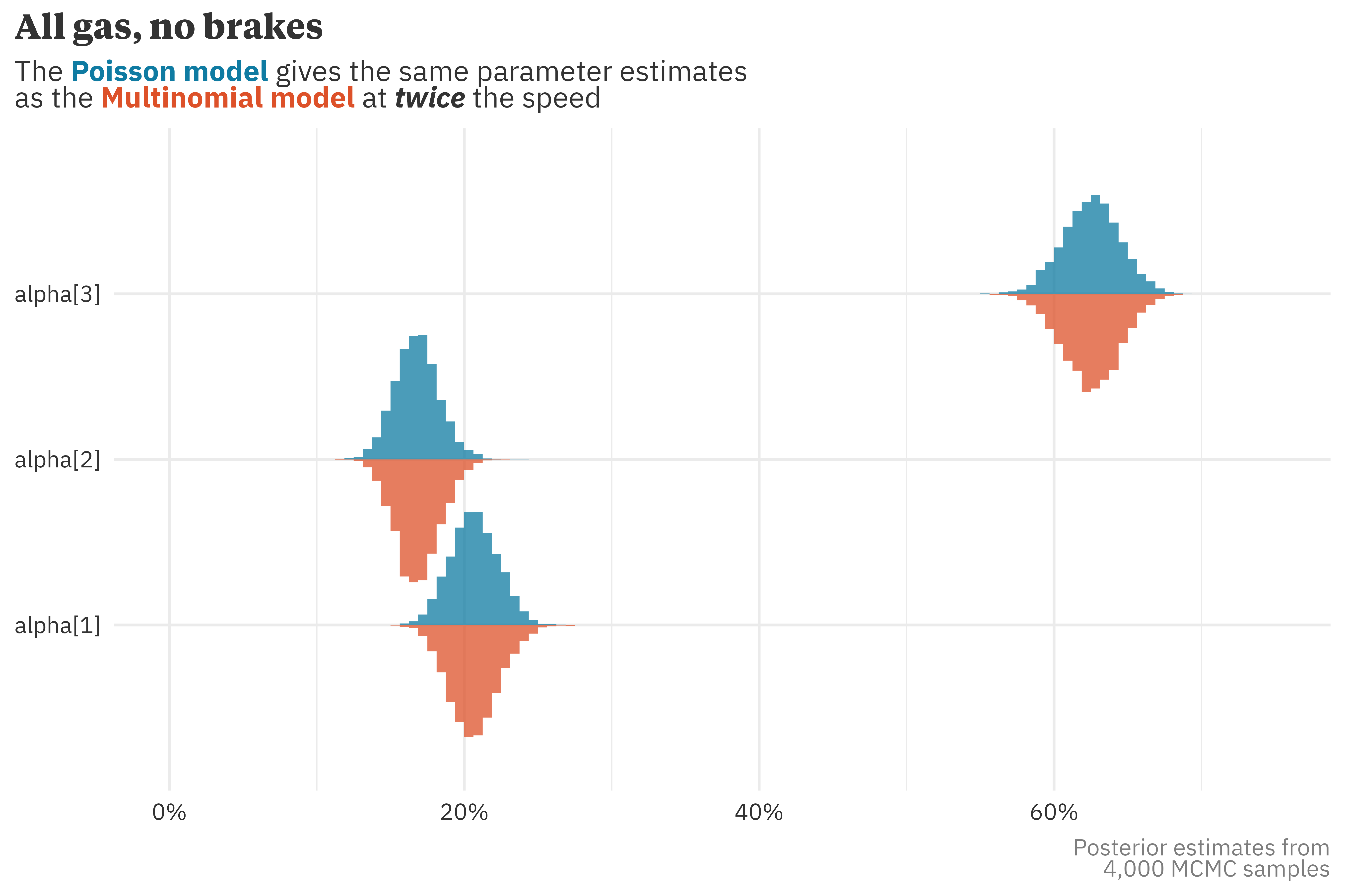
  • I’d mentioned this before but it’s worth repeating: the benefits of vectorization truly are a free lunch! We get the same parameter estimates from both models at roughly twice the speed!6

  • 6 In this toy example, the sampling time roughly halves. In larger, complex models I’ve built in practice, I’ve seen sampling times drop by 75% with a Poisson implementation.

  • Code
    multinomial_draws <- 
      multinomial_fit$draws(format = "df") |> 
      pivot_longer(starts_with("alpha"),
                   names_to = "variable",
                   values_to = "estimate") |>
      mutate(model = "multinomial_implementation") |>
      select(model, .draw, variable, estimate)
    
    poisson_draws <- 
      poisson_fit$draws(format = "df") |>
      pivot_longer(starts_with("alpha"),
                   names_to = "variable",
                   values_to = "estimate") |>
      mutate(model = "poisson_implementation") |>
      select(model, .draw, variable, estimate)
    
    poisson_draws |>
      bind_rows(multinomial_draws) |>
      mutate(side = if_else(model == "poisson_implementation", "top", "bottom")) |> 
      ggplot(aes(x = variable,
                 y = estimate,
                 fill = model,
                 color = model,
                 side = side)) + 
      stat_histinterval(slab_alpha = 0.75,
                        scale = 0.75,
                        alpha = 0,
                        breaks = seq(from = 0, to = 0.75, by = 0.00625)) +
      scale_y_percent() + 
      MetBrewer::scale_fill_met_d("Egypt") + 
      coord_flip() +
      theme_rieke() +
      theme(legend.position = "none") +
      labs(title = glue::glue("**All gas, no brakes**"),
           subtitle = glue::glue("The ",
                                 "**{color_text('Poisson model', MetBrewer::MetPalettes$Egypt[[1]][2])}** ",
                                 "gives the same parameter estimates <br>as the ",
                                 "**{color_text('Multinomial model', MetBrewer::MetPalettes$Egypt[[1]][1])}** ",
                                 "at **_twice_** the speed"),
           x = NULL,
           y = NULL,
           caption = "Posterior estimates from<br>4,000 MCMC samples")

    Citation

    BibTeX citation:
    @online{rieke2023,
      author = {Rieke, Mark},
      title = {Free Lunch at the Vectorization Table},
      date = {2023-04-26},
      url = {https://www.thedatadiary.net/posts/2023-04-25-zoom-zoom},
      langid = {en}
    }
    
    For attribution, please cite this work as:
    Rieke, Mark. 2023. “Free Lunch at the Vectorization Table.” April 26, 2023. https://www.thedatadiary.net/posts/2023-04-25-zoom-zoom.

    Stay in touch

    Support my work with a coffee

    Share