Sufficiently Normal

library(tidyverse)
library(cmdstanr)
library(ggdist)
library(riekelib)

# Setup a color palette to be used for groups A/B
pal <- NatParksPalettes::NatParksPalettes$Acadia[[1]][c(2,8)]

As a somewhat unexpected follow-up to my previous post on the sufficient gamma, I’ve decided to take a similarly motivated look at implementing the sufficient normal. I’d previously implemented the sufficient normal as a part of my March Madness predictions last year,¹ but if I’m being honest, I got that working without getting an intuition for why it worked. That’s bugged me for the better part of a year, so here we are.

¹ My current employer is a subsidiary of LV Sands, so it is unlikely that I put together a model for March Madness this year.

Like last time, if you want to skip the derivation and just get right to implementation, here’s a sufficient normal density function that you can drop right at the top of your Stan model:

real sufficient_normal_lpdf(
  real Xsum,
  real Xsumsq,
  real n,
  real mu,
  real sigma
) {
  real lp = 0.0;
  real s2 = sigma^2;
  real d = (2 * s2)^(-1);
  lp += -n * 0.5 * log(2 * pi() * s2);
  lp += -d * Xsumsq;
  lp += 2 * d * mu * Xsum;
  lp += -n * d * mu^2;
  return lp;
}

Notably Normal

I’ll simulate 5,000 observations from two normally distributed groups for a total of 10,000 observations in the dataset. I’ll then fit two models to these 10,000 observations — one making use of Stan’s built-in normal likelihood and another with our custom sufficient normal density function.

set.seed(2026)
normal_data <-
  tibble(group = c("A", "B"),
         mu = c(0, 2),
         sigma = c(1, 0.5)) %>%
  mutate(y = pmap(list(mu, sigma), ~rnorm(5000, ..1, ..2)))

normal_data %>%
  unnest(y) %>%
  ggplot(aes(x = y,
             y = group,
             fill = group)) +
  stat_histinterval(breaks = 60,
                    slab_alpha = 0.75) +
  scale_fill_manual(values = pal) +
  theme_rieke()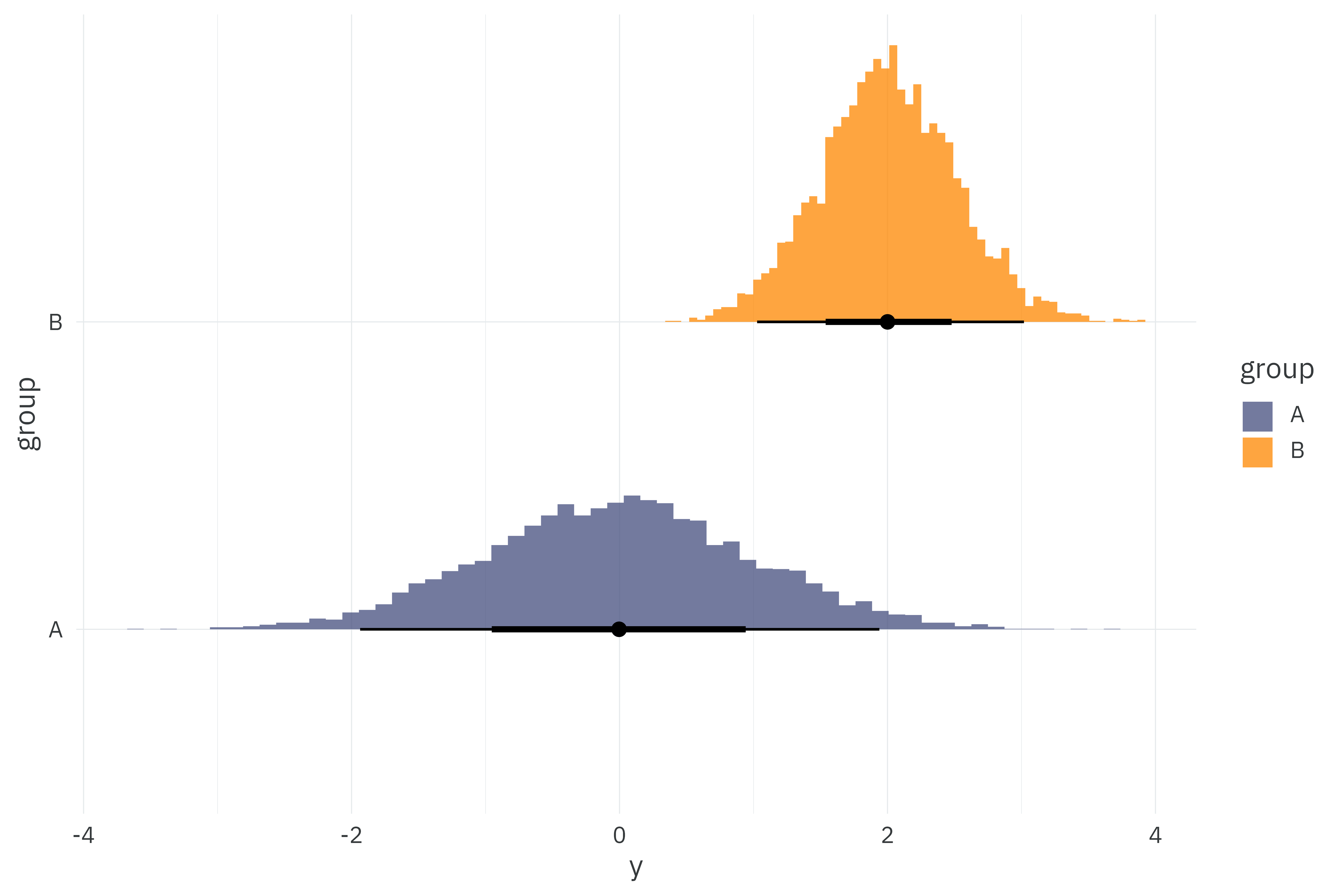

We’ll fit a simple normal likelihood to these observations where each group, $g$, has a separate mean, $\mu$, and standard deviation, $\sigma$. Unsurprisingly, this model fits with no issues.

$$\begin{array}{rl}{y}_i& \sim \mathcal{N}({\mu }_g,{\sigma }_g)\\ {\mu }_g& \sim \mathcal{N}(0,5)\\ {\sigma }_g& \sim \text{Exponential}(1)\end{array}$$

data {
  // Dimensions
  int<lower=0> N;                          // Number of observations
  int G;                                   // Number of groups

  // Observations
  vector[N] Y;                             // Outcome per observation
  array[N] int<lower=1, upper=G> gid;      // Group membership per observation
  
  // Normal priors
  real mu_mu;
  real<lower=0> sigma_mu;
  real<lower=0> lambda_sigma;
}

parameters {
  vector[G] mu;
  vector<lower=0>[G] sigma;
}

model {
  target += normal_lpdf(mu | mu_mu, sigma_mu);
  target += exponential_lpdf(sigma | lambda_sigma);
  for (n in 1:N) {
    target += normal_lpdf(Y[n] | mu[gid[n]], sigma[gid[n]]);
  }
}

individual_model <- cmdstan_model("individual-normal.stan")

model_data <-
  normal_data %>%
  mutate(gid = rank(group)) %>%
  unnest(y)

stan_data <-
  list(
    N = nrow(model_data),
    Y = model_data$y,
    G = max(model_data$gid),
    gid = model_data$gid,
    mu_mu = 0,
    sigma_mu = 5,
    lambda_sigma = 1
  )

start_time <- Sys.time()
individual_fit <-
  individual_model$sample(
    data = stan_data,
    seed = 1234,
    iter_warmup = 1000,
    iter_sampling = 1000,
    chains = 10,
    parallel_chains = 10
  )
run_time_individual <- as.numeric(Sys.time() - start_time)

plot_posterior <- function(fit) {
  
  # Get the true parameters used in simulation
  truth <-
    normal_data %>%
    select(group, mu, sigma) %>%
    pivot_longer(-group,
                 names_to = "parameter",
                 values_to = "draw") %>%
    mutate(parameter = if_else(parameter == "mu", "\u03bc", "\u03c3"))
  
  fit$draws(c("mu", "sigma"), format = "df") %>%
    as_tibble() %>%
    select(starts_with("mu"), starts_with("sigma")) %>%
    pivot_longer(everything(),
                 names_to = "parameter",
                 values_to = "draw") %>%
    nest(data = -parameter) %>%
    separate(parameter, c("parameter", "group"), "\\[") %>%
    mutate(group = str_remove(group, "\\]"),
           group = if_else(group == "1", "A", "B"),
           parameter = if_else(parameter == "mu", "\u03bc", "\u03c3")) %>%
    unnest(data) %>%
    ggplot(aes(x = draw,
               y = parameter,
               fill = group)) +
    stat_histinterval(breaks = 60,
                      slab_alpha = 0.75) +
    geom_point(data = truth,
               color = "red") +
    scale_fill_manual(values = pal) +
    theme_rieke()
  
}

plot_posterior(individual_fit) +
  labs(title = "**Fit against individual observations**",
       subtitle = "Can be used as a baseline for evaluating the sufficient formulation",
       x = NULL,
       y = NULL)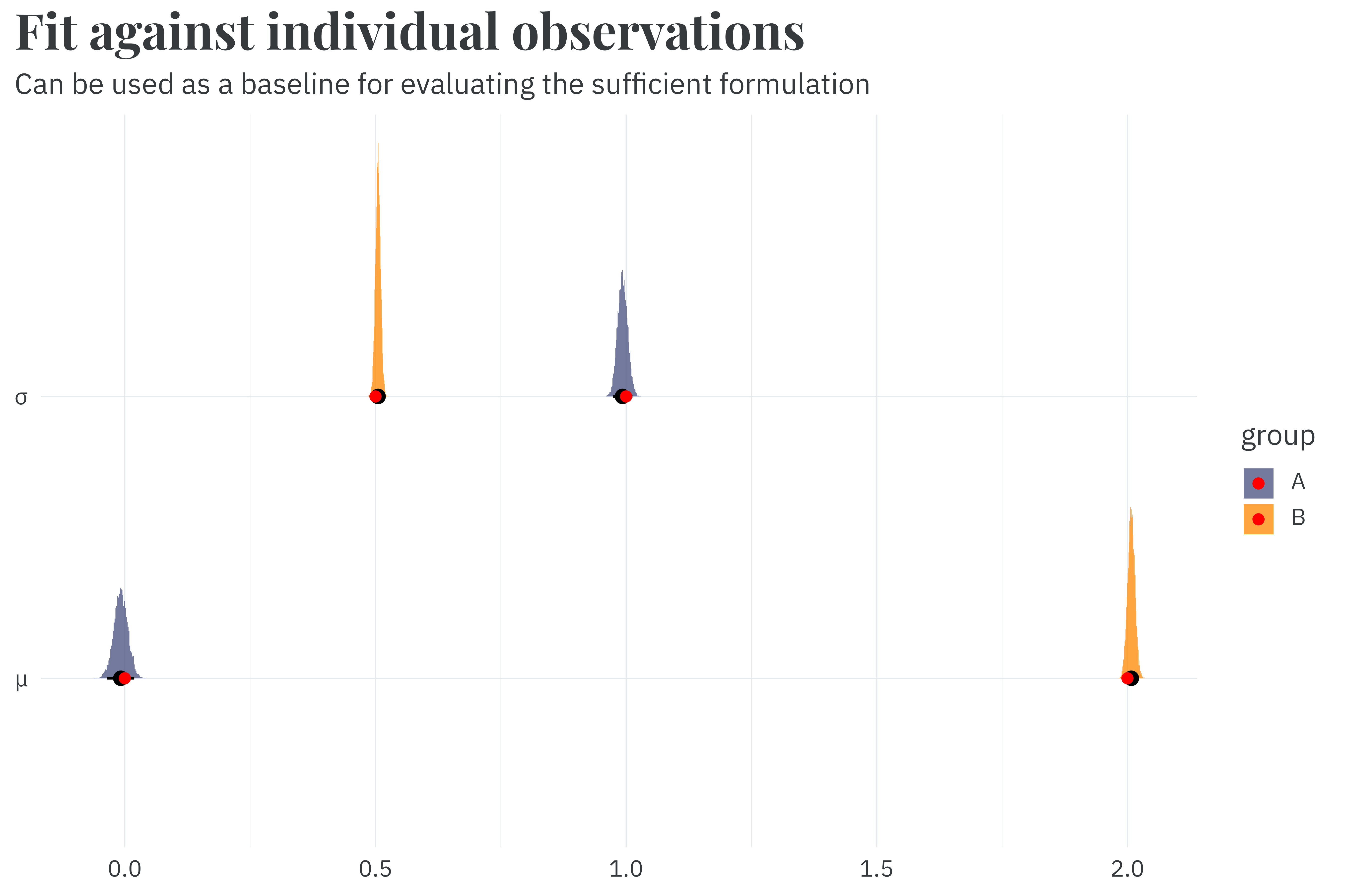

While it only takes 4.1 seconds to fit this model,² we have some room for improvement by summarizing the dataset with a sufficient formulation.

² As an aside, wow Stan’s implementation of the normal likelihood is incredibly fast.

Density Derivations

When fitting a model, we repeatedly multiply the probability density for each individual observation to get a total probability density for the entire set of observations. A sufficient exploit would allow us to calculate this product in one step, rather than repeatedly calculating the individual probability densities.

$$\begin{array}{rl}Pr(y_1,y_2,\dots ,y_n)& =Pr(y_1)Pr(y_2)\dots Pr(y_n)\\ Pr(y)& =\prod _i^{N}Pr(y_i)\end{array}$$

The probability density of the normal distribution with mean $\mu$ and standard deviation $\sigma$ for a single observation $y_i$ is:

$$Pr(y_i)=\frac{1}{\sqrt{2\pi {\sigma }^2}}{e}^{\frac{1}{2{\sigma }^2}(y_i-\mu {)}^2}$$

Our goal is to find a variant of this density function that allows us to evaluate $\prod Pr(y)$ given summary information from $y$, rather than individual observations. Bayesian models evaluate log probabilities and it’s generally easier to work on the log scale — the log of the normal density function for a single observation is:

$$\log (Pr(y_i))=-\frac{1}{2}\log (2\pi {\sigma }^2)-\frac{(y_i-\mu {)}^2}{2{\sigma }^2}$$

We want to setup $y_i$ in such a way that we can easily replace it with summary statistics when we move from a single observation to multiple observations. Here, that means we need to expand $(y_i-\mu {)}^2$.

$$\begin{array}{rl}\log (Pr(y_i))& =-\frac{1}{2}\log (2\pi {\sigma }^2)-\frac{y_i^2-2\mu y_i+{\mu }^2}{2{\sigma }^2}\\ & =-\frac{1}{2}\log (2\pi {\sigma }^2)-(2{\sigma }^2{)}^{-1}(y_i^2-2\mu y_i+{\mu }^2)\end{array}$$

The last step of this expansion is to multiply $(2{\sigma }^2{)}^{-1}$ by each of the quadratic terms. For legibility’s sake (and to save some keystrokes), I set $d=(2{\sigma }^2{)}^{-1}$. We end up with the following equation for the log-probability of a single observation, $y_i$.

$$\begin{array}{rl}\log (Pr(y_i))& =-\frac{1}{2}\log (2\pi {\sigma }^2)-d{y}_i^2+2d\mu y_i-d{\mu }^2\end{array}$$

The simplest case beyond a single observation is to consider two observations. Because we’re on the log scale we can simply add the two together to get the log of the product.

$$\begin{array}{rl}\log (Pr(y_1,y_2))=& -\frac{1}{2}\log (2\pi {\sigma }^2)-d{y}_1^2+2d\mu y_1-d{\mu }^2\\ & -\frac{1}{2}\log (2\pi {\sigma }^2)-d{y}_2^2+2d\mu y_2-d{\mu }^2\end{array}$$

This framing makes it clear how this product expands to $n$ observations. For each observation, we have another set of $\frac{1}{2}\log (2\pi {\sigma }^2)$ and $d{\mu }^2$ terms, so we can simply multiply these terms by $n$. Each $y_i^2$ term is multiplied by $d$, so we replace $d(y_1^2+y_2^2\cdots +y_n^2)$ with $d\sum y^2$ (and can do the same operation to get to $2d\mu \sum y$). Altogether, we arrive at a new log probability function based on the count, sum, and sum of square terms in $y$.

$$\log (Pr(y))=-\frac{n}{2}\log (2\pi {\sigma }^2)-d\sum y^2+2d\mu \sum y-nd{\mu }^2$$

The log probability is what Stan uses during sampling and is how I defined the function in the intro of this article. For completeness’ sake, we can unlog to show that the probability density of a normally distributed set of observations, $y$, has a sufficient formulation given the count, sum, and sum of squares in $y$.

$$Pr(\sum y^2,\sum y,n|\mu ,\sigma )=\frac{1}{(2\pi {\sigma }^2{)}^{n/2}}{e}^{(-2{\sigma }^2{)}^{-1}(\sum y^2-2\mu \sum y+n{\mu }^2)}$$

Sufficient Speedups

With this sufficient formulation, we can collapse our original 10,000 row dataset into just two rows — one per group.

sufficient_model <- cmdstan_model("sufficient-normal.stan")

model_data <-
  normal_data %>%
  mutate(gid = rank(group),
         n = map_int(y, length),
         Ysum = map_dbl(y, sum),
         Ysumsq = map_dbl(y, ~sum(.x^2)))

model_data

#> # A tibble: 2 × 8
#>   group    mu sigma y               gid     n    Ysum Ysumsq
#>   <chr> <dbl> <dbl> <list>        <dbl> <int>   <dbl>  <dbl>
#> 1 A         0   1   <dbl [5,000]>     1  5000   -40.3  4927.
#> 2 B         2   0.5 <dbl [5,000]>     2  5000 10039.  21429.

We can keep the same priors and just swap out our original likelihood function for our new sufficient likelihood.

$$\begin{array}{rl}\sum y^2,\sum y,n& \sim \text{Sufficient-Normal}({\mu }_g,{\sigma }_g)\\ {\mu }_g& \sim \mathcal{N}(0,5)\\ {\sigma }_g& \sim \text{Exponential}(1)\end{array}$$

functions {
  real sufficient_normal_lpdf(
    real Xsum,
    real Xsumsq,
    real n,
    real mu,
    real sigma
  ) {
    real lp = 0.0;
    real s2 = sigma^2;
    real d = (2 * s2)^(-1);
    lp += -n * 0.5 * log(2 * pi() * s2);
    lp += -d * Xsumsq;
    lp += 2 * d * mu * Xsum;
    lp += -n * d * mu^2;
    return lp;
  }
}

data {
  // Dimensions
  int<lower=0> N;                          // Number of observations
  int G;                                   // Number of groups

  // Observations
  vector[N] Ysum;                          // Sum of a group of observations
  vector[N] Ysumsq;                        // Sum(y^2) of a group of observations
  vector[N] n_obs;                         // Number of observations per group
  array[N] int<lower=1, upper=G> gid;      // Group membership
  
  // Normal priors
  real mu_mu;
  real<lower=0> sigma_mu;
  real<lower=0> lambda_sigma;
}

parameters {
  vector[G] mu;
  vector<lower=0>[G] sigma;
}

model {
  target += normal_lpdf(mu | mu_mu, sigma_mu);
  target += exponential_lpdf(sigma | lambda_sigma);
  for (n in 1:N) {
    target += sufficient_normal_lpdf(Ysum[n] | Ysumsq[n], n_obs[n], mu[gid[n]], sigma[gid[n]]);
  }
}

stan_data <-
  list(
    N = nrow(model_data),
    Ysum = model_data$Ysum,
    Ysumsq = model_data$Ysumsq,
    n_obs = model_data$n,
    G = max(model_data$gid),
    gid = model_data$gid,
    mu_mu = 0,
    sigma_mu = 5,
    lambda_sigma = 1
  )

start_time <- Sys.time()
sufficient_fit <-
  sufficient_model$sample(
    data = stan_data,
    seed = 1234,
    iter_warmup = 1000,
    iter_sampling = 1000,
    chains = 10,
    parallel_chains = 10
  )
run_time_sufficient <- as.numeric(Sys.time() - start_time)

Fitting the sufficient formulation to the same dataset only takes 0.7 seconds, a 5.6x speedup compared to the fit against individual observations.³ And we recover the same posterior that we see in the fit against individual observations!

³ Because the normal likelihood in Stan is already so optimized, this isn’t as large of a speedup as we saw in the sufficient gamma. But in both cases, the speedup from sufficiency is largely determined by the original dataset’s size. For example, fitting the original model to 200,000 individual observations takes ~90s, whereas it still only takes ~0.7 in the sufficient model.

plot_posterior(sufficient_fit)  +
  labs(title = "**Fit using the sufficient normal**",
       subtitle = "Recovers the same posterior from the fit to individual observations!",
       x = NULL,
       y = NULL)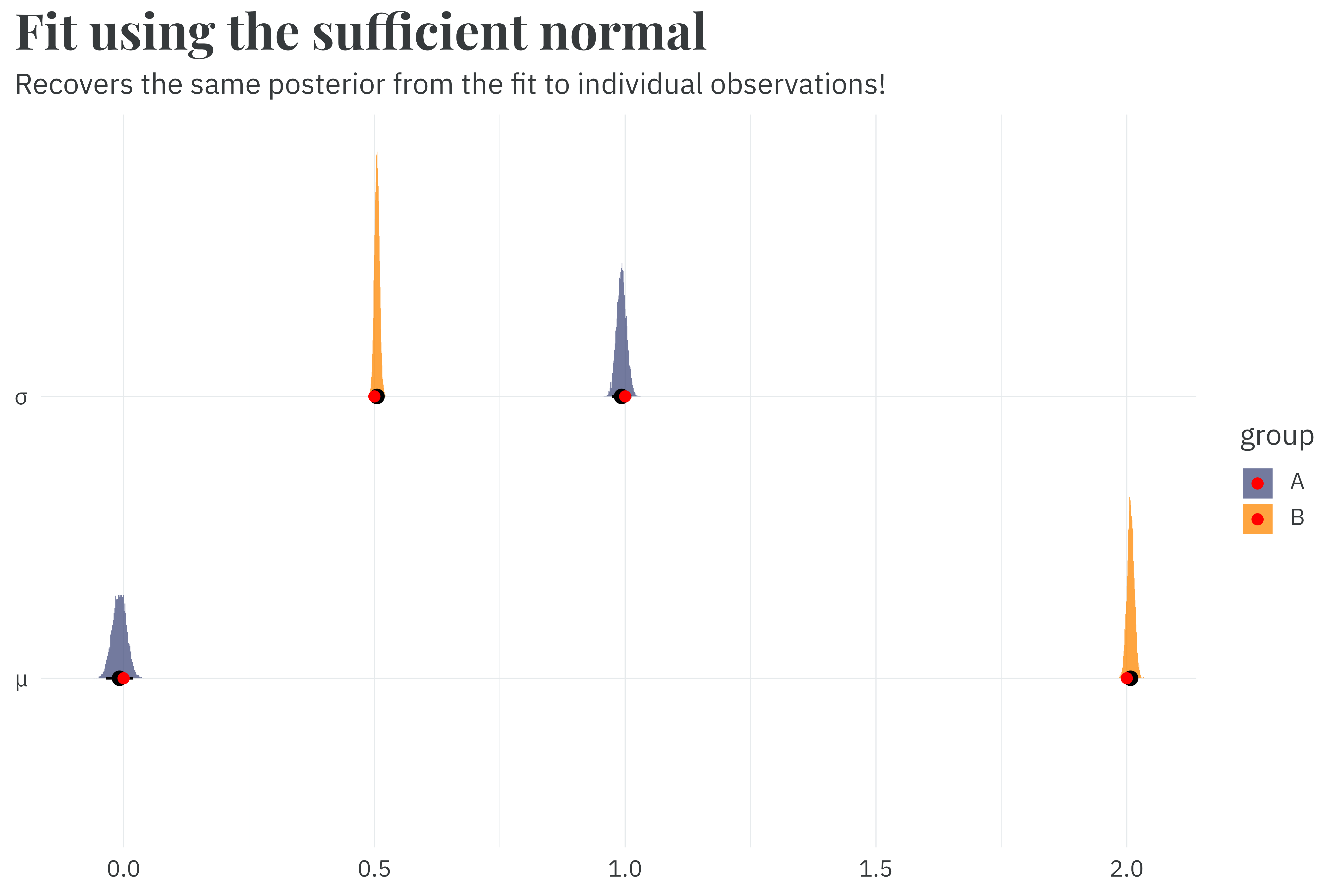

Once again, exploit sufficiency, go zoom zoom. I simply must be cannot be stopped.