Multivariate Madness

Note

In accordance with my AI policy, I have written this post with the assistance of a LLM. All text in this post is written by me, but I had some assistance from a LLM beboppin’ to help work through the matrix manipulations as a part of the sufficiency derivation.

library(tidyverse)
library(cmdstanr)
library(ggdist)
library(riekelib)
library(patchwork)

# Setup a color palette to be used for groups A/B
pal <- NatParksPalettes::NatParksPalettes$Acadia[[1]][c(2,8)]

Sometimes, an idea takes hold in such a way that it fully consumes you, taking over every free thought. And even when focus is diverted elsewhere, the idea sits in the back of your mind, lurking, waiting. For the last few months, one such idea has existed for me: making models go zoom via sufficiency exploits. I’ve previously written about sufficient formulations for gamma, normal, and poisson likelihoods. Here, we break free from the shackles of a single dimension. Here, there are no gods. Here, there are no masters. Here, I introduce a sufficient formulation of the multivariate normal.

As in previous posts, if you want to skip the derivation,¹ you can just drop this sufficient multivariate normal density function at the top of your Stan model. Here, xxts is the element-wise sum \(\sum \mathbf{y}\mathbf{y}^\text{T}\),² xts is the element-wise sum \(\sum \mathbf{y}^\text{T}\), and \(n\) is the number of observations.

¹ Though why would you, when the derivation will leave you in a state such as this:

² I, for some reason, default to using x for variable names in functions even when used for response variables. Very cool! Very consistent!

real multi_normal_sufficient_lpdf(
  matrix xxts,
  row_vector xts,
  real n,
  vector mu,
  matrix Sigma
) {
  int K = size(mu);
  matrix[K,K] invs = inverse(Sigma);
  real lp = 0.0;
  lp += (-n * K) / 2 * log(2 * pi());
  lp += -n/2 * log_determinant(Sigma);
  lp += -0.5 * trace(Sigma \ xxts);
  lp += trace(invs * mu * xts);
  lp += -n/2 * (mu' * invs * mu);
  return lp;
}

Into the Multiverse

We’ll simulate 5,000 observations from two bivariate-normal distributed groups, each with known means, marginal standard deviations, and covariances. We’ll then fit two models to these 10,000 observations — one making use of Stan’s built-in multivariate normal likelihood and another with the custom sufficient density function above.

set.seed(2026)
mvn_data <-
  tibble(group = c("A", "B"),
         mu = list(c(0, 2), c(-2, 1)),
         sigma = list(c(0.25, 1), c(0.5, 0.75)),
         rho = c(0.8, -0.4)) %>%
  mutate(Sigma = pmap(list(sigma, rho),
                      ~matrix(c(..1[1]^2, prod(..1) * ..2, prod(..1) * ..2, ..1[2]^2),
                              nrow = 2)),
         y = pmap(list(mu, Sigma), ~MASS::mvrnorm(5000, ..1, ..2))) 

mvn_data %>%
  mutate(y = map(y, ~as_tibble(.x, .name_repair = "universal"))) %>%
  unnest(y) %>%
  rename(y1 = `...1`,
         y2 = `...2`) %>%
  ggplot(aes(x = y1,
             y = y2,
             color = group)) + 
  geom_point(alpha = 0.25,
             shape = 21) +
  scale_color_manual(values = pal) +
  theme_rieke()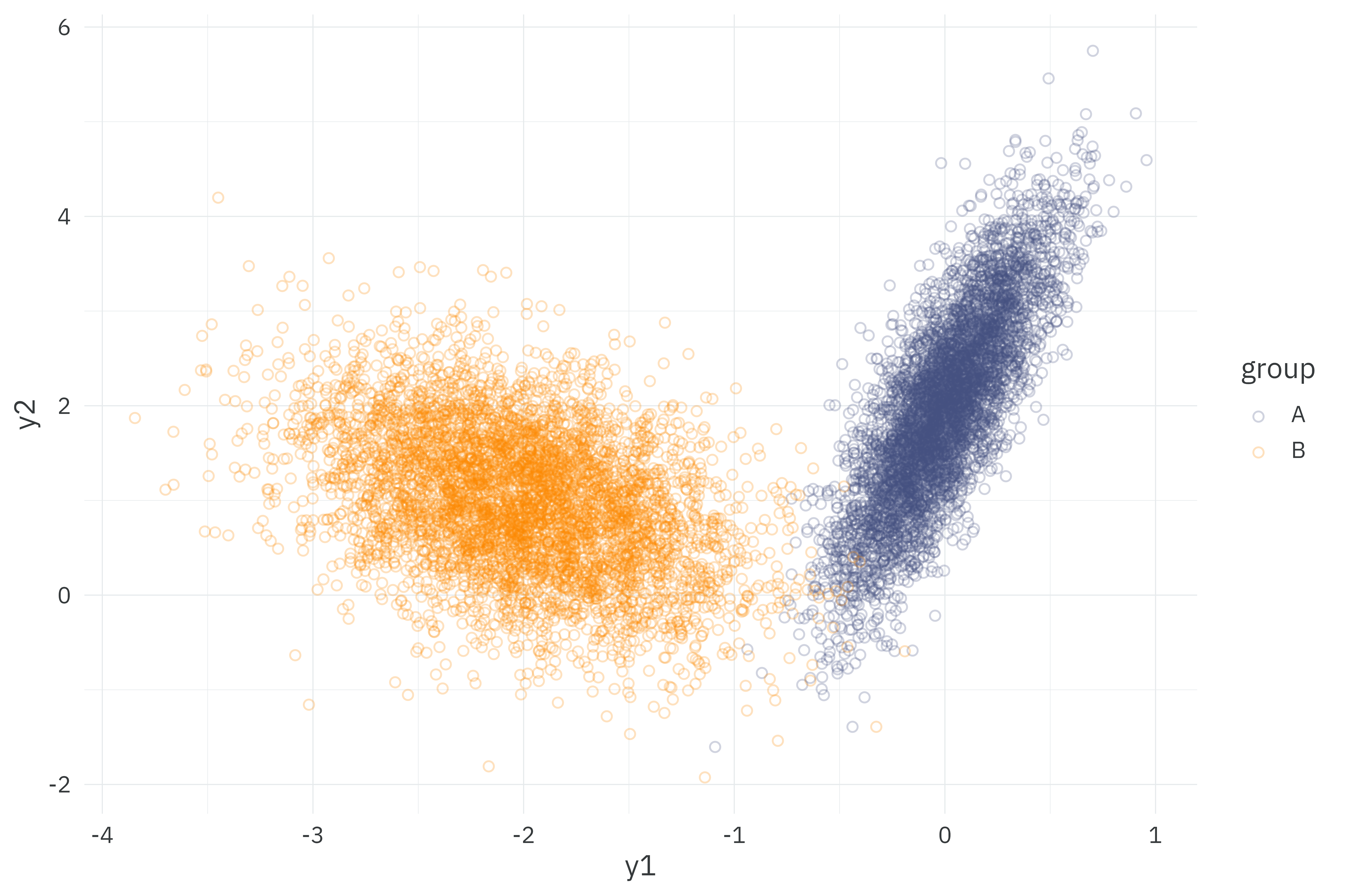

We’ll fit a multivariate normal likelihood to these observations where each group, \(g\), has a separate mean vector, \(\boldsymbol{\mu}\), and covariance matrix, \(\mathbf{\Sigma}\). The covariance matrix is derived from marginal standard deviations, \(\sigma\), and correlation, \(\rho\). The model itself is fit using the LKJ prior but we compute the fitted \(\rho\) in the generated quantities block in order to compare against the value used to simulate the data.³

³ Judge me not for the triple-nested for loop in the generated quantities block.

\[ \begin{align*} \mathbf{y}_i &\sim \text{Multi-Normal}(\boldsymbol{\mu}_g, \mathbf{\Sigma}_g) \\ \boldsymbol{\mu}_g &= \begin{bmatrix} \mu_{g,1} \\ \mu_{g,2} \end{bmatrix} \\ \mathbf{\Sigma}_g &= \mathbf{L}_g \times \mathbf{L}_g^{\text{T}} \\ \mathbf{L}_g &= \text{diag}(\boldsymbol{\sigma}_g) \times \mathbf{L}_{\text{corr}, g} \\ \boldsymbol{\sigma}_g &= \begin{bmatrix} \sigma_{g,1} \\ \sigma_{g,2} \end{bmatrix} \\ \mu_{g,i} &\sim \mathcal{N}(0,5) \\ \sigma_{g,i} &\sim \text{Exponential}(1) \\ \mathbf{L}_{\text{corr},g} &\sim \text{LKJ-Cholesky}(2) \end{align*} \]

data {
  // Dimensions
  int<lower=0> N;                          // Number of observations
  int<lower=1> K;                          // Number of dimensions observed
  int G;                                   // Number of groups

  // Observations
  array[N] vector[K] Y;                    // Outcome per observation
  array[N] int<lower=1, upper=G> gid;      // Group membership per observation
  
  // Multi-normal priors
  real mu_mu;
  real<lower=0> sigma_mu;
  real<lower=0> lambda_sigma;
  real<lower=0> lkj_prior;
}

parameters {
  array[G] vector[K] mu;
  array[G] vector[K] sigma;
  array[G] cholesky_factor_corr[K] L_corr;
}

transformed parameters {
  array[G] cholesky_factor_cov[K] L;
  array[G] matrix[K, K] Sigma;
  for (g in 1:G) {
    L[g] = diag_pre_multiply(sigma[g], L_corr[g]);
    Sigma[g] = multiply_lower_tri_self_transpose(L[g]);
  }
}

model {
  for (g in 1:G) {
    target += normal_lpdf(mu[g] | mu_mu, sigma_mu);
    target += exponential_lpdf(sigma[g] | lambda_sigma);
    target += lkj_corr_cholesky_lpdf(L_corr[g] | lkj_prior);
  }
  
  for (n in 1:N) {
    target += multi_normal_cholesky_lpdf(Y[n] | mu[gid[n]], L[gid[n]]);
  }
}

generated quantities {
  array[G] matrix[K, K] rho;
  for (g in 1:G) {
    for (i in 1:K) {
      for (j in 1:K) {
        rho[g,i,j] = Sigma[g,i,j] / (sigma[g,i] * sigma[g,j]);
      }
    }
  }
}

individual_model <- cmdstan_model("individual-mvn.stan")

model_data <- 
  mvn_data %>%
  mutate(gid = rank(group),
         y = map(y, ~as_tibble(.x, .name_repair = "universal"))) %>%
  unnest(y) %>%
  rename(y1 = `...1`,
         y2 = `...2`)

stan_data <-
  list(
    N = nrow(model_data),
    K = length(mvn_data$mu[[1]]),
    Y = cbind(model_data$y1, model_data$y2),
    G = max(model_data$gid),
    gid = model_data$gid,
    mu_mu = 0,
    sigma_mu = 5,
    lambda_sigma = 1,
    lkj_prior = 2
  )

start_time <- as.numeric(Sys.time())
individual_fit <-
  individual_model$sample(
    data = stan_data,
    seed = 1234,
    iter_warmup = 1000,
    iter_sampling = 1000,
    chains = 10,
    parallel_chains = 10
  )
run_time_individual <- as.numeric(Sys.time()) - start_time

plot_posterior <- function(fit) {
  
  truth <- 
    mvn_data %>%
    select(group, mu, sigma, rho) %>%
    mutate(rho = map(rho, ~.x)) %>%
    pivot_longer(c(mu, sigma, rho),
                 names_to = "parameter",
                 values_to = "draw") %>%
    mutate(parameter = case_when(parameter == "mu" ~ "\u03bc",
                                 parameter == "sigma" ~ "\u03c3",
                                 parameter == "rho" ~ "\u03c1"),
           parameter_group = parameter,
           kid = map(draw, ~1:length(.x))) %>%
    unnest(c(draw, kid)) %>%
    mutate(parameter = if_else(parameter != "\u03c1",
                               paste0(parameter, "<sub>", kid, "</sub>"),
                               parameter))
  
  fit$draws(c("mu", "sigma", "rho"), format = "df") %>%
    as_tibble() %>%
    select(starts_with("mu"), starts_with("sigma"), starts_with("rho")) %>%
    pivot_longer(everything(),
                 names_to = "parameter",
                 values_to = "draw") %>%
    filter(str_detect(parameter, "mu|sigma|,1,2]")) %>%
    nest(data = -parameter) %>%
    mutate(parameter = if_else(str_detect(parameter, "rho"),
                               str_replace(parameter, ",1,2", ""),
                               parameter),
           group = if_else(str_detect(parameter, "\\[1"), "A", "B"),
           kid = if_else(str_detect(parameter, ",1"), 1, 2),
           kid = if_else(str_detect(parameter, "rho"), NA, kid),
           parameter = str_extract(parameter, "mu|sigma|rho"),
           parameter = case_when(parameter == "mu" ~ "\u03bc",
                                 parameter == "sigma" ~ "\u03c3",
                                 parameter == "rho" ~ "\u03c1"),
           parameter_group = parameter,
           parameter = if_else(parameter != "\u03c1",
                               paste0(parameter, "<sub>", kid, "</sub>"),
                               parameter)) %>%
    unnest(data) %>%
    ggplot(aes(x = draw,
               y = parameter,
               fill = group)) +
    stat_histinterval(slab_alpha = 0.75) +
    geom_point(data = truth,
               color = "red") +
    scale_fill_manual(values = pal) +
    facet_wrap(~parameter_group, scales = "free", ncol = 1) +
    theme_rieke() +
    theme(axis.text.y.left = ggtext::element_markdown(color = "#363a3c"))
  
}

plot_posterior(individual_fit) +
  labs(title = "**Fit against individual observations**",
       subtitle = "Can be used as a baseline for evaluating the sufficient formulation",
       x = NULL,
       y = NULL)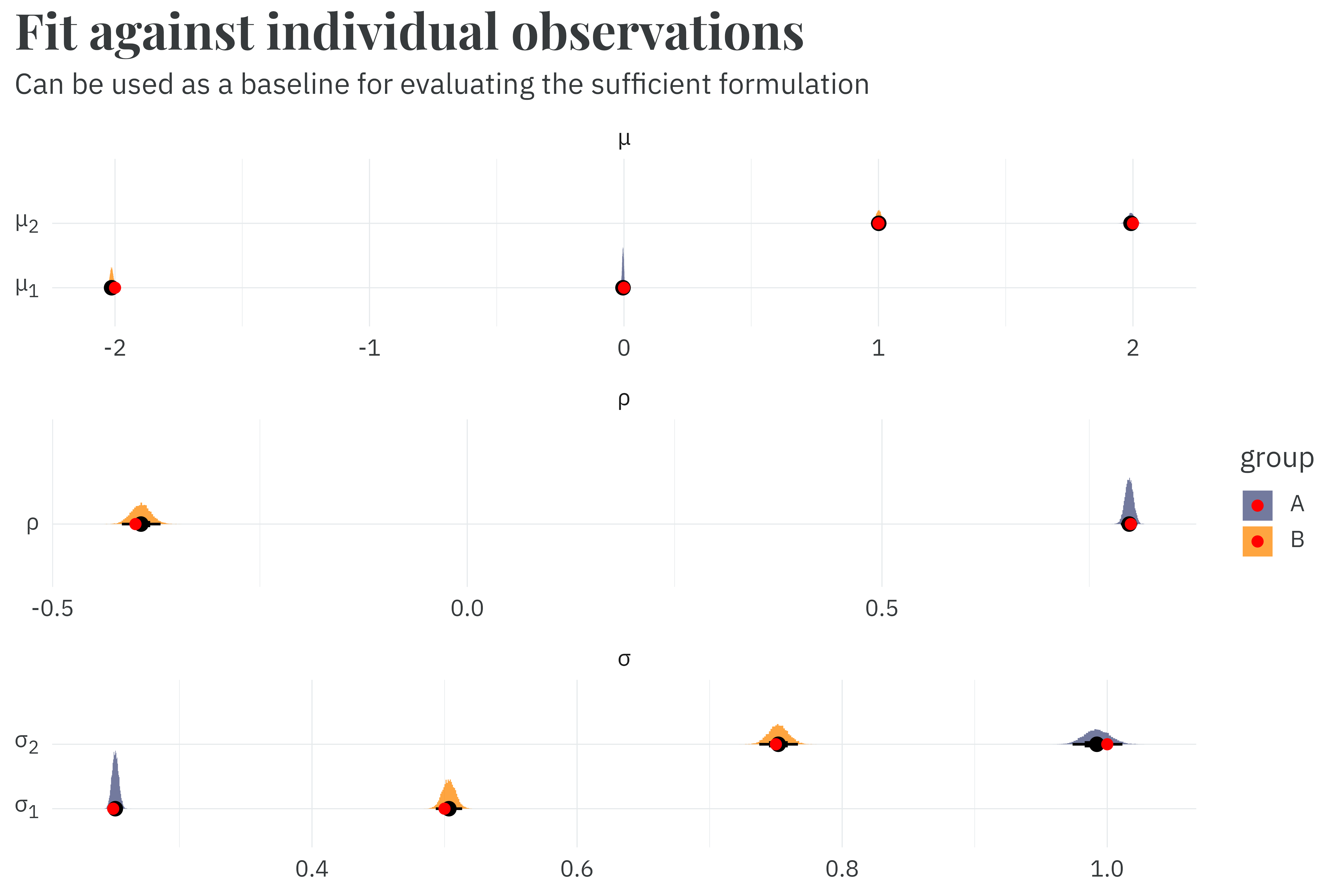

This implementation takes 110.0 seconds to fit. While not fast, it recovers the parameters used to simulate the data. Rather than throwing more compute at the problem, we can speed this up by being smarter about our implementation.

A Delusional Descent into Density Derivation Delerium

Our basic strategy stays the same from that used in previous entries in this series on sufficiency: convert repeated multiplications of the probability density function for individual observations into a single equation that calculates the product for all observations in one fell swoop.

\[ \begin{align*} \Pr(y_1,y_2,\dots,y_n) &= \Pr(y_1)\Pr(y_2)\dots\Pr(y_n) \\ \Pr(y) &= \prod_i^N \Pr(y_i) \end{align*} \]

The probability density function of the multivariate normal distribution with mean vector \(\boldsymbol{\mu}\) and covariance matrix \(\mathbf{\Sigma}\) for a single observation vector \(\mathbf{y}_i\) is:

\[ \Pr(\mathbf{y}_i) = (2 \pi)^{-k/2} \det(\mathbf{\Sigma})^{-1/2} \exp\left(\frac{(\mathbf{y}_i - \boldsymbol{\mu})^\text{T}\mathbf{\Sigma}^{-1}(\mathbf{y}_i - \boldsymbol{\mu})}{2}\right) \]

Stan and other probabilistic programming languages work by finding parameters that maximize the probability density function of the observed data.⁴ This is generally⁵ easier on the log scale, so we’ll work with the log of the density function. If we collapse the mess of matrices and vectors on the right hand side of the equation into \(\eta\), the log of the multivariate normal density function for a single observation becomes:

⁴ I’m sweeping a bunch of cool details about how samplers work under the rug but, like, chill.

⁵ Always?

\[ \begin{align*} \log(\Pr(\mathbf{y}_i)) &= -\frac{k}{2} \log(2 \pi) - \frac{1}{2}\log(\det(\mathbf{\Sigma})) - \frac{1}{2}\underbrace{(\mathbf{y}_i - \boldsymbol{\mu})^\text{T}\mathbf{\Sigma}^{-1}(\mathbf{y}_i - \boldsymbol{\mu})}_{\eta_i} \\ &= -\frac{k}{2} \log(2 \pi) - \frac{1}{2}\log(\det(\mathbf{\Sigma})) - \frac{1}{2}\eta_i \end{align*} \]

The first step towards finding a general sufficient solution is to consider the simplest case beyond a single observation: two observations. Because we’re on the log scale we can simply add the two together to get the log of the product.

\[ \begin{align*} \log(\Pr(\mathbf{y}_1,\mathbf{y}_2)) = &-\frac{k}{2} \log(2 \pi) - \frac{1}{2}\log(\det(\mathbf{\Sigma})) - \frac{1}{2}\eta_1 \\ &-\frac{k}{2} \log(2 \pi) - \frac{1}{2}\log(\det(\mathbf{\Sigma})) - \frac{1}{2}\eta_2 \end{align*} \]

Moving beyond two observations is as simple as repeatedly adding to the log probability. At \(n\) observations, we simply multiply the first two terms by \(n\) and find the sum of \(\eta\) for each element in \(\mathbf{y}\). Already, this is most⁶ of the work towards a sufficient formulation of the multivariate normal. We just need to deal with that pesky \(\eta\) term where our data, \(\mathbf{y}\), actually live.

⁶ Well. Not really most. But the version of me that drafted the body of this post was a lot pluckier than the current version of me who had to deal with all the bugs and wonkiness I encountered during implementation. Harumph.

\[ \log(\Pr(\mathbf{y})) = -\frac{nk}{2} \log(2 \pi) - \frac{n}{2}\log(\det(\mathbf{\Sigma})) - \frac{1}{2}\sum \eta_i \]

Much like in scalar algebra, matrix multiplication is distributive. We can expand \(\eta\) from a single product into four additive terms.⁷

⁷ FOIL, anyone?

\[ \begin{align*} \eta_i &= (\mathbf{y}_i - \boldsymbol{\mu})^\text{T} \mathbf{\Sigma}^{-1} (\mathbf{y}_i - \boldsymbol{\mu}) \\ &= (\mathbf{y}_i^\text{T} - \boldsymbol{\mu}^\text{T}) \mathbf{\Sigma}^{-1} (\mathbf{y}_i - \boldsymbol{\mu}) \\ &= \mathbf{y}_i^\text{T} \mathbf{\Sigma}^{-1} (\mathbf{y}_i - \boldsymbol{\mu}) - \boldsymbol{\mu}^\text{T} \mathbf{\Sigma}^{-1} (\mathbf{y}_i - \boldsymbol{\mu}) \\ &= \left(\mathbf{y}_i^\text{T} \mathbf{\Sigma}^{-1} \mathbf{y}_i\right) - \left(\mathbf{y}_i^\text{T} \mathbf{\Sigma}^{-1} \boldsymbol{\mu}\right) - \left(\boldsymbol{\mu}^\text{T} \mathbf{\Sigma}^{-1} \mathbf{y}_i\right) + \left(\boldsymbol{\mu}^\text{T} \mathbf{\Sigma}^{-1} \boldsymbol{\mu}\right) \end{align*} \]

Each of these term in the expansion results in a scalar value. The transpose of a scalar value is equivalent to the scalar value itself. We can also “distribute” the transposition to find:

\[ \begin{align*} \mathbf{y}_i^\text{T} \mathbf{\Sigma}^{-1} \boldsymbol{\mu} &= \left(\mathbf{y}_i^\text{T} \mathbf{\Sigma}^{-1} \boldsymbol{\mu}\right)^\text{T} \\ &= \boldsymbol{\mu}^\text{T} \mathbf{\Sigma}^{-1} \mathbf{y}_i \end{align*} \]

Subbing this in for one of the middle terms lets us shrink the equation for \(\eta\) from four terms to three.

\[ \eta_i = \left(\mathbf{y}_i^\text{T} \mathbf{\Sigma}^{-1} \mathbf{y}_i\right) - 2 \left(\mathbf{y}_i^\text{T} \mathbf{\Sigma}^{-1} \boldsymbol{\mu}\right) + \left(\boldsymbol{\mu}^\text{T} \mathbf{\Sigma}^{-1} \boldsymbol{\mu}\right) \]

We need to get all of our data, \(\mathbf{y}\), cleanly separated from the model’s parameters \(\boldsymbol{\mu}\) and \(\mathbf{\Sigma}\). This will allow us to pass in summary data for \(\mathbf{y}\) without having to know anything about the parameters. As it stands now, our terms for \(\mathbf{y}\) are tightly wound up with the parameters. To decouple data and parameters, we’ll take a momentary diversion into the world of traces.

The trace of a matrix is just the sum of the values along the diagonal.

\[ \text{tr}(\mathbf{A}) = \sum_{i=1}^{K} \mathbf{A}_{i,i} \]

Conveniently, traces have the property that the trace of a matrix product can be rearranged, provided that order is preserved.

\[ \text{tr}(\mathbf{ABC}) = \text{tr}(\mathbf{BCA}) = \text{tr}(\mathbf{CAB}) \]

The trace of a scalar value is just the value itself. Because each term in \(\eta\) is a scalar, we can set it to the trace of itself then rearrange within the trace to get the \(\mathbf{y}\) components butting-up against one another.

\[ \begin{align*} \mathbf{y}_i^\text{T} \mathbf{\Sigma}^{-1} \mathbf{y}_i &= \text{tr}\left(\mathbf{y}_i^\text{T} \mathbf{\Sigma}^{-1} \mathbf{y}_i\right) \\ &= \text{tr}\left(\mathbf{\Sigma}^{-1} \mathbf{y}_i \mathbf{y}_i^\text{T}\right) \end{align*} \]

Rather than summing up individual observations, we can replace \(\mathbf{y}_i\mathbf{y}_i^\text{T}\) with its element-wise sum, \(\sum\mathbf{y}\mathbf{y}^\text{T}\), which can be pre-computed outside of the model.

\[ \sum \mathbf{y}^\text{T} \mathbf{\Sigma}^{-1} \mathbf{y} = \text{tr}\left(\mathbf{\Sigma}^{-1} \sum \mathbf{y} \mathbf{y}^\text{T} \right) \]

We can perform a similar set of operations to rearrange the second term in \(\eta\) and summarize with a sum that can be computed outside of the model.⁸

⁸ Did I realize that \(\mathbf{y}\) was already separable from the parameters after I wrote this section and implemented the trace as a part of the sufficient likelihood function. Yes. Am I going to go back and change it? No.

\[ \begin{align*} \mathbf{y}_i^\text{T} \mathbf{\Sigma}^{-1} \boldsymbol{\mu} &= \text{tr}\left(\mathbf{y}_i^\text{T} \mathbf{\Sigma}^{-1} \boldsymbol{\mu}\right) \\ &= \text{tr}\left(\mathbf{\Sigma}^{-1} \boldsymbol{\mu} \mathbf{y}_i^\text{T}\right) \\ \\ \sum \mathbf{y}^\text{T} \mathbf{\Sigma}^{-1} \boldsymbol{\mu} &= \text{tr}\left(\mathbf{\Sigma}^{-1} \boldsymbol{\mu} \sum \mathbf{y} \right) \end{align*} \]

The third term in \(\eta\) does not depend on data in \(\mathbf{y}\), so for \(n\) observations we simply multiply the term by \(n\). Altogether, our new equation for \(\sum \eta\) becomes:

\[ \sum \eta = \text{tr}\left(\mathbf{\Sigma}^{-1} \sum \mathbf{y} \mathbf{y}^\text{T} \right) - 2\ \text{tr}\left(\mathbf{\Sigma}^{-1} \boldsymbol{\mu} \sum \mathbf{y}^\text{T} \right) + n \left(\boldsymbol{\mu}^\text{T} \mathbf{\Sigma}^{-1} \boldsymbol{\mu} \right) \]

Subbing this in to the original log density function (and distributing \(\frac{1}{2}\) across the individual terms in \(\sum \eta\)) yields the following beautiful monstrosity of a sufficient function for the log-probability of a multivariate normal.⁹

⁹ Just look at this lovecraftian beast. It’ll drive you mad.

\[ \begin{align*} \log(\Pr(\mathbf{y}, n \mid \boldsymbol{\mu}, \mathbf{\Sigma})) = &-\frac{nk}{2} \log(2 \pi) \\ &-\frac{n}{2} \log(\det(\mathbf{\Sigma})) \\ &-\frac{1}{2} \text{tr} \left(\mathbf{\Sigma}^{-1} \sum \mathbf{y} \mathbf{y}^\text{T} \right) \\ &+\text{tr} \left(\mathbf{\Sigma}^{-1} \boldsymbol{\mu} \sum \mathbf{y}^\text{T} \right) \\ &-\frac{n}{2} \left(\boldsymbol{\mu}^\text{T} \mathbf{\Sigma}^{-1} \boldsymbol{\mu}\right) \end{align*} \]

Sufficient Speedups

With this sufficient formulation, we can collapse our original 10,000 row dataset into just two rows — one per group. \(\sum\mathbf{y}\mathbf{y}^\text{T}\) and \(\sum\mathbf{y}^\text{T}\) are computed from data ahead of time and are passed to the model as a matrix and vector, respectively.

sufficient_model <- cmdstan_model("sufficient-mvn.stan")

xxt <- function(x) {
  return(x %*% t(x))
}

yyts <- function(y) {
  out <- matrix(0, nrow = 2, ncol = 2)
  for (i in 1:length(y[,1])) {
    out <- out + xxt(y[i,])
  }
  return(out)
}

yts <- function(y) {
  out <- c(0, 0)
  for (i in 1:length(y[,1])) {
    out <- out + y[i,]
  }
  return(out)
}

model_data <-
  mvn_data %>%
  mutate(yyts = map(y, yyts),
         yts = map(y, yts),
         n_obs = map_dbl(y, nrow),
         gid = rank(group))

model_data %>%
  select(group, gid, yyts, yts, n_obs)

#> # A tibble: 2 × 5
#>   group   gid yyts          yts       n_obs
#>   <chr> <dbl> <list>        <list>    <dbl>
#> 1 A         1 <dbl [2 × 2]> <dbl [2]>  5000
#> 2 B         2 <dbl [2 × 2]> <dbl [2]>  5000

We can keep the same priors and just swap out our original likelihood function for our new sufficient likelihood.

\[ \begin{align*} \sum\mathbf{y}\mathbf{y}^\text{T}, \sum\mathbf{y}^\text{T}, n &\sim \text{Sufficient-Multi-Normal}(\boldsymbol{\mu}_g, \mathbf{\Sigma}_g) \\ \boldsymbol{\mu}_g &= \begin{bmatrix} \mu_{g,1} \\ \mu_{g,2} \end{bmatrix} \\ \mathbf{\Sigma}_g &= \mathbf{L}_g \times \mathbf{L}_g^{\text{T}} \\ \mathbf{L}_g &= \text{diag}(\boldsymbol{\sigma}_g) \times \mathbf{L}_{\text{corr}, g} \\ \boldsymbol{\sigma}_g &= \begin{bmatrix} \sigma_{g,1} \\ \sigma_{g,2} \end{bmatrix} \\ \mu_{g,i} &\sim \mathcal{N}(0,5) \\ \sigma_{g,i} &\sim \text{Exponential}(1) \\ \mathbf{L}_{\text{corr},g} &\sim \text{LKJ-Cholesky}(2) \end{align*} \]

functions {
  real multi_normal_sufficient_lpdf(
    matrix xxts,
    row_vector xts,
    real n,
    vector mu,
    matrix Sigma
  ) {
    int K = size(mu);
    matrix[K,K] invs = inverse(Sigma);
    real lp = 0.0;
    lp += (-n * K) / 2 * log(2 * pi());
    lp += -n/2 * log_determinant(Sigma);
    lp += -0.5 * trace(Sigma \ xxts);
    lp += trace(invs * mu * xts);
    lp += -n/2 * (mu' * invs * mu);
    return lp;
  }
}

data {
  // Dimensions
  int<lower=0> N;                          // Number of observations
  int<lower=1> K;                          // Number of dimensions observed
  int G;                                   // Number of groups

  // Observations
  array[N] matrix[K,K] yyts;               // Element-wise sum(y * y') for all y in Y
  array[N] row_vector[K] yts;              // Element-wise sum(y') for all y in Y
  vector[N] n_obs;                         // Number of observations per group
  array[N] int<lower=1, upper=G> gid;      // Group membership per observation

  // Multi-normal priors
  real mu_mu;
  real<lower=0> sigma_mu;
  real<lower=0> lambda_sigma;
  real<lower=0> lkj_prior;
}

parameters {
  array[G] vector[K] mu;
  array[G] vector[K] sigma;
  array[G] cholesky_factor_corr[K] L_corr;
}

transformed parameters {
  array[G] cholesky_factor_cov[K] L;
  array[G] matrix[K, K] Sigma;
  for (g in 1:G) {
    L[g] = diag_pre_multiply(sigma[g], L_corr[g]);
    Sigma[g] = multiply_lower_tri_self_transpose(L[g]);
  }
}

model {
  for (g in 1:G) {
    target += normal_lpdf(mu[g] | mu_mu, sigma_mu);
    target += exponential_lpdf(sigma[g] | lambda_sigma);
    target += lkj_corr_cholesky_lpdf(L_corr[g] | lkj_prior);
  }
  
  for (n in 1:N) {
    target += multi_normal_sufficient_lpdf(yyts[n] | yts[n], n_obs[n], mu[gid[n]], Sigma[gid[n]]);
  }
}

generated quantities {
  array[G] matrix[K, K] rho;
  for (g in 1:G) {
    for (i in 1:K) {
      for (j in 1:K) {
        rho[g,i,j] = Sigma[g,i,j] / (sigma[g,i] * sigma[g,j]);
      }
    }
  }
}

stan_data <- 
  list(
    N = nrow(model_data),
    K = length(mvn_data$mu[[1]]),
    G = max(model_data$gid),
    yyts = model_data$yyts,
    yts = model_data$yts,
    n_obs = model_data$n_obs,
    gid = model_data$gid,
    mu_mu = 0,
    sigma_mu = 5,
    lambda_sigma = 1,
    lkj_prior = 2
  )

start_time <- as.numeric(Sys.time())
sufficient_fit <-
  sufficient_model$sample(
    data = stan_data,
    seed = 1234,
    iter_warmup = 1000,
    iter_sampling = 1000,
    chains = 10,
    parallel_chains = 10
  )
run_time_sufficient <- as.numeric(Sys.time()) - start_time

Fitting the sufficient formulation to the same dataset only takes 0.9 seconds, a 116.0x speedup compared to the fit against individual observations. And since the sufficient formulation is doing the exact same math under the hood we get the exact same posterior on the other side.

plot_posterior(sufficient_fit)  +
  labs(title = "**Fit using the sufficient multivariate normal**",
       subtitle = "Recovers the same posterior from the fit to individual observations!",
       x = NULL,
       y = NULL)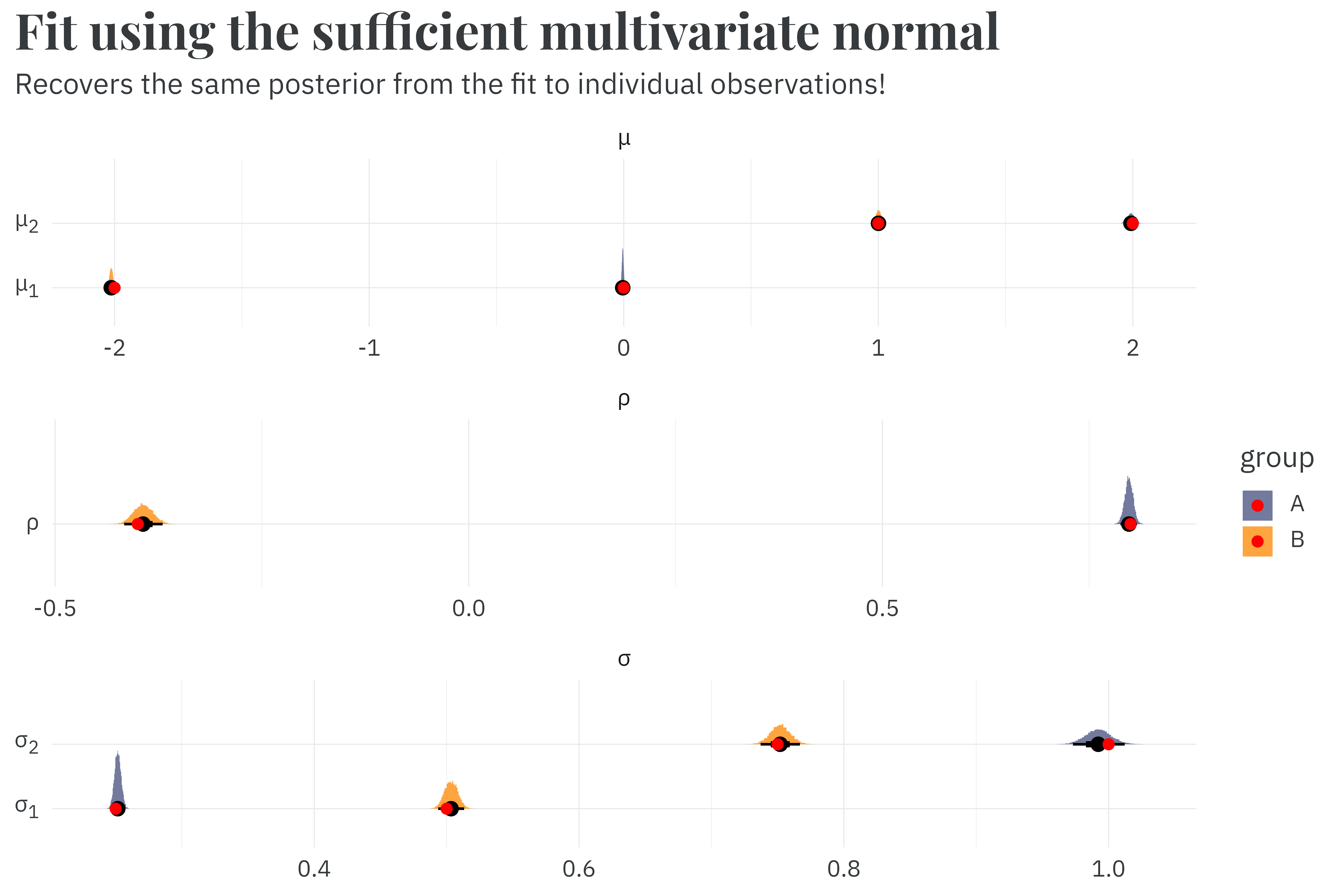

This might be one of the coolest things I’ve ever done. It may have also driven me to madness. Worth it.