Churn, baby, churn

Code

library(tidyverse)
library(riekelib)
library(cmdstanr)

Understanding the average customer lifetime is crucial for businesses as it provides valuable insights into customer behavior and the overall health of the customer base. It’s a critical component of revenue forecasting and estimating the average customer lifetime value and can also be used to highlight opportunities for product improvement. Average customer lifetime is also connected to customer churn rates — if the churn rate is known, you can calculate the average customer lifetime.¹

¹ Under the assumption that the churn rate is constant over time. More on that later.

Estimating the churn rate from customer data is an interesting modeling problem. A simple average of the churn rate among customers who have churned will overestimate the churn rate — this average excludes active customers who will (potentially) remain active for a long time! A better method is to estimate churn via censored regression, which can account for observations with missing (i.e., censored) events (in this case, the churn date for active customers).² Censored models, however, make some assumptions that can conflict with the reality of data collection. Namely, censored models assume that time is continuous and no events occur at \(t = 0\).

² These are also called survival models. I assume this is because they’re also used in measuring the effect of clinical treatments on a patient’s expected remaining lifetime. I prefer to call them censored models because it describes the data more accurately. Plus it’s a bit less morbid.

In reality, data is often recorded in discrete time. For example, if I look at when customers drop out of a subscription service, the data may be grouped by day, month, quarter, or year. A censored model assumes that the data is continuous, rather than grouped.³ Additionally, when measured in discrete time, churn data can include events at \(t=0\). In the subscription service example, if the data were grouped by month, we may observe some customers that cancel their subscription prior to month end. These customers never made it to the end of the month (\(t=1\)), so their churn is recorded during month \(0\).

³ A sufficient number of discrete time groups approximates continuous time, but when there are few time periods, this approximation can fall apart a bit.

As an alternative to a traditional censored model, I’ll present a modified censored model that estimates the probability of an event occurring in a discrete time period as the probability that the event occurs between two points in continuous time. This modification naturally accounts for the case when an event occurs at \(t=0\). I’ll build up to this model over the course of applying several faulty models to simulated data of player churn after the launch of a new mobile game. The discrete censored model should recover the simulated churn rate and can be used to estimate the average player lifetime.

Deriving average customer lifetime

Let’s suppose that one million players download and play a new mobile game on launch day. If we assume that 15% of players will stop playing each day, the number of daily players over the first fifteen days might look like this:

Code

# set parameters
n_players <- 1e6
churn_rate <- 0.15
n_days <- 15

# simulate daily number of active players
set.seed(12345)
days <- 0:n_days
active_players <- vector(length = length(days))
active_players[1] <- n_players
for (d in 2:length(days)) {
  active_players[d] <- rbinom(1, active_players[d - 1], (1 - churn_rate))
}

# how we might pull from a curated table
player_data <- 
  tibble(day = days,
         players = active_players) 

# plot!
player_data %>%
  ggplot(aes(x = day,
             y = players)) + 
  geom_col(fill = "royalblue",
           alpha = 0.75) +
  scale_y_comma() +
  theme_rieke() +
  labs(title = "**Number of daily active players**",
       subtitle = glue::glue("Given an initial player base of **",
                             scales::label_comma()(n_players),
                             "** and a **",
                             scales::label_percent(accuracy = 1)(churn_rate),
                             "** churn rate."),
       x = "Days since install",
       y = NULL)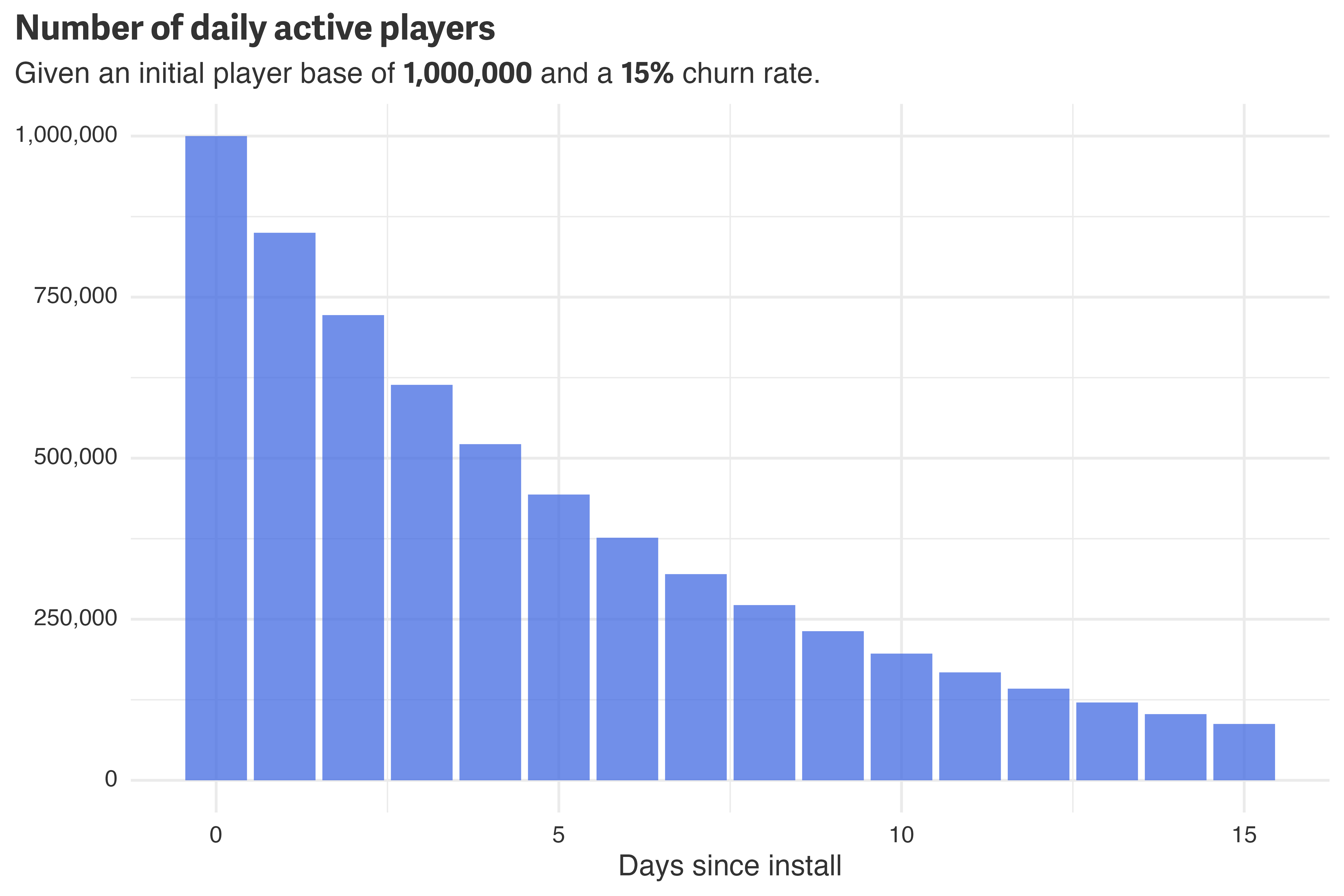

Despite having an initial player base of one million players, by the fifteenth day, there are fewer than one-hundred thousand active players! Given this data, we may want to answer two questions: What is the churn rate? and What is the average customer lifetime? I manually set the churn rate to 15%, but we’ll need to do some work to derive the average customer lifetime.

The active players on any given day was simulated as a draw from a binomial distribution. The number of trials is the number of active players on the previous day, \(\text{Players}_{\text{day}[d-1]}\), and the probability of success, \(\theta\), is given as \(1-R\), where \(R\) is the churn rate.

\[ \begin{align*} \text{Players}_{\text{day}[d]} &\sim \text{Binomial}(\text{Players}_{\text{day}[d-1]}, \theta) \\ \theta &= 1 - R \end{align*} \]

The expected value from this distribution is then the probability of success multiplied by the number of trials.

\[ \begin{align*} \hat{\text{Players}_{\text{day}[d]}} &= \text{Players}_{\text{day}[d-1]} \times (1 - R) \end{align*} \]

If we want to know the expected number of players on day two, we first need the expected number of players on day one. Since day one is dependent on day 0, we can recursively plug-in the same equation for \(\text{Players}_{\text{day}[1]}\). Simplifying shows that the number of active players on day two is only dependent on the initial number of players, the churn rate, and the number of days in between.

\[ \begin{align*} \hat{\text{Players}_{\text{day}[2]}} &= \text{Players}_{\text{day}[1]} \times (1 - R) \\ &= [\text{Players}_{\text{day}[0]} \times (1 - R)] \times (1 - R) \\ &= \text{Players}_{\text{day}[0]} \times (1-R)^2 \end{align*} \]

This equation can be generalized to estimate the expected number of players on any day, \(d\) by recursively multiplying the initial player base by \((1 - R)\).⁴

⁴ As we’ll see later, this sort of recursive multiplication suggests that \(e\) is hiding out somewhere in our equation.

\[ \hat{\text{Players}_{\text{day}[d]}} = \text{Players}_{\text{day}[0]} \times (1 - R)^d \]

Dividing by the initial player population gives the proportion of players remaining on day \(d\).

\[ \frac{\text{Players}_{\text{day}[d]}}{\text{Players}_{\text{day}[0]}} = (1 - R)^d \]

Plotting this over each day, \(d\), yields something resembling a survival curve.

Code

tibble(x = 0:90) %>%
  mutate(y = (1 - churn_rate)^x) %>%
  ggplot(aes(x = x,
             y = y)) + 
  geom_line(color = "royalblue") +
  scale_y_percent() +
  theme_rieke() +
  labs(title = "**Expected proportion of remaining players**",
       subtitle = glue::glue("Given a **",
                             scales::label_percent(accuracy = 1)(churn_rate),
                             "** churn rate"),
       x = "Days since install",
       y = NULL)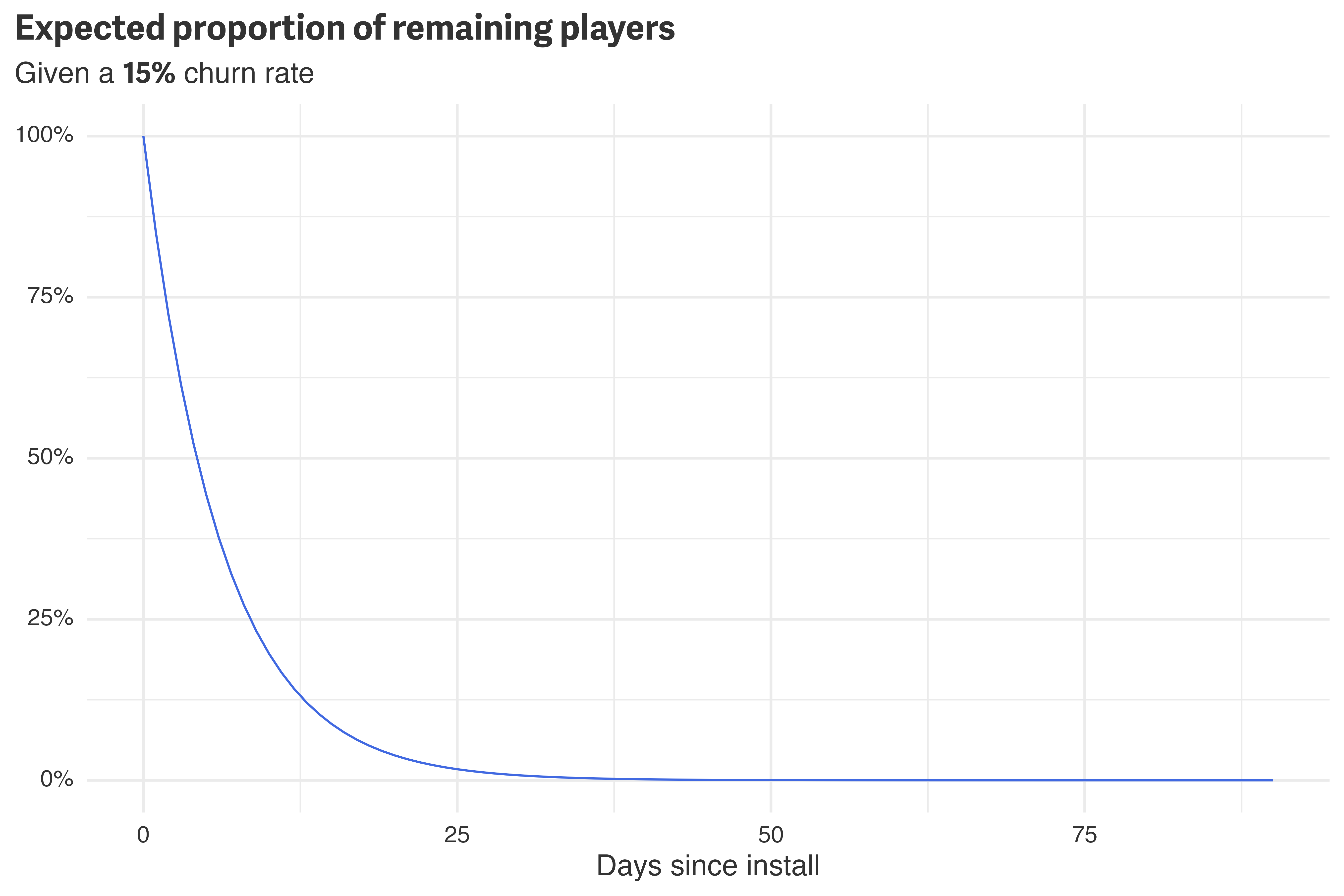

Since the proportion is unitless, integrating over days gives the “average number of days.” This is exactly what we’re looking for — the average customer lifetime (in days).⁵

⁵ I had to break out the good ’ole integration tables for this one, but look! I found \(e\)!

\[ \begin{align*} \text{Average Customer Lifetime} &= \int_0^\infty (1 - R)^d \text{d}d \\ \text{Average Customer Lifetime} &= \frac{-1}{\log(1 - R)} \end{align*} \]

Since the churn rate \(R\) is known to be 15%, the average customer lifetime in this example is just 6.2 days. When the churn rate isn’t known, however, we can estimate it with a model.

Modeling churn

Model 1: Binomial

Suppose the churn rate is not known and instead all we have is the daily active player data (in this case, 15 days worth). The first few rows of the dataset show that the playerbase is declining day-over-day:

Code

player_data %>%
  mutate(across(everything(), ~scales::label_comma()(.x))) %>%
  rename(Day = day,
         `Active Players` = players) %>%
  slice_head(n = 5) %>%
  knitr::kable()

Day	Active Players
0	1,000,000
1	849,938
2	722,133
3	613,865
4	521,802

A reasonable first pass at a model definition would be to model the daily number of active players as a binomial where the number of trials is the number of active players on the previous day. In fact, this is exactly how the simulated data were created.

\[ \begin{align*} \text{Players}_{\text{day}[d]} &\sim \text{Binomial}(\text{Players}_{\text{day}[d-1]}, \theta) \\ \theta &= 1 - R \\ R &\sim \text{Beta}(1, 1) \end{align*} \]

While this process can be used to simulate data, it causes problems when modeling. Namely, this model grossly overstates the number of observations that are in the dataset. For a player to be a part of \(\text{Players}_{\text{day}[d-1]}\), they must also be a part of \(\text{Player}_{\text{day}[d-2]}, \ \text{Player}_{\text{day}[d-3]}, \ \dots, \ \text{Player}_{\text{day}[0]}\). This player gets counted as \(d-1\) observations!

For example, to pass data to this model, we’d need a slight variation of the dataset:

Code

player_data %>%
  mutate(players_lag = lag(players)) %>%
  drop_na() %>%
  mutate(across(everything(), ~scales::label_comma()(.x))) %>%
  rename(Day = day,
         `Players [d]` = players,
         `Players [d-1]` = players_lag) %>%
  slice_head(n = 4) %>%
  knitr::kable()

Day	Players [d]	Players [d-1]
1	849,938	1,000,000
2	722,133	849,938
3	613,865	722,133
4	521,802	613,865

The total number of observations in this model is the sum of the column Players [d-1]. In this case, despite there only being one million players, this model would have 6,081,336 observations!

A more reasonable alternative would be to model the number of players on a specific day, \(d=D\).

\[ \begin{align*} \text{Players}_{\text{day}[D]} &\sim \text{Binomial}(\text{Players}_{\text{day}[0]}, \theta_D) \\ \theta_D &= (1 - R)^D \\ R &\sim \text{Beta}(1, 1) \end{align*} \]

Code

data {
  int<lower=1> D;                // day to evaluate
  int<lower=0> K;                // number of active players on day 0
  int<lower=0, upper=K> S;       // number of active players on day D 
}
parameters {
  real<lower=0, upper=1> churn_rate;
}
transformed parameters {
  real<lower=0, upper=1> theta = (1 - churn_rate)^D;
}
model {
  // priors
  churn_rate ~ beta(1, 1);
  
  // likelihood
  S ~ binomial(K, theta);
}
generated quantities {
  real average_lifetime = -1/log(1 - churn_rate);
}

In this model, the number of observations according to the model matches reality: one million players. The downside, however, is that this model is only able to show information about the specific day, \(D\) — it assumes that the churn rate is constant.⁶ Regardless, fitting this model for \(d = 10\) recovers the churn rate and average customer lifetime.

⁶ In this case, this happens to be a really good assumption, since I simulated the data with a constant churn rate. But that isn’t always the case! Other models are better equipped to handle constant or varying churn rates.

Code

# day to evaluate
D <- 10

# number of "successes" on day 
S <- 
  player_data %>%
  filter(day == D) %>%
  pull(players)

# data for the model
binomial_data <-
  list(
    D = D,
    K = n_players,
    S = S
  )

# compile, fit, & display output
binomial_model <-
  cmdstan_model("binomial_churn.stan")

binomial_fit <- 
  binomial_model$sample(
    data = binomial_data,
    iter_warmup = 1000,
    iter_sampling = 1000,
    chains = 4,
    parallel_chains = 4,
    seed = 987
  )

binomial_fit$summary() %>%
  filter(variable %in% c("churn_rate", "average_lifetime")) %>%
  select(variable, median, q5, q95) %>%
  knitr::kable()

variable	median	q5	q95
churn_rate	0.150094	0.149815	0.150373
average_lifetime	6.148955	6.136569	6.161380

Model 2: Censored Regression

The binomial model worked well in this case, but a better approach would be to estimate the churn day for each player directly. This provides a way to incorporate each day into the model without overestimating the number of observations in the dataset. Given the simulated dataset, a plot of the number of churns per day is visually similar to the number of active players per day, but the scale is much smaller.

Code

player_data %>%
  mutate(churned = players - lead(players)) %>%
  ggplot(aes(x = day,
             y = churned)) +
  geom_col(fill = "royalblue",
           alpha = 0.75) +
  scale_y_comma() + 
  theme_rieke() +
  labs(title = "**Number of churns per day**",
       subtitle = glue::glue("From an initial player base of **",
                             scales::label_comma()(n_players),
                             "**"),
       x = "Days since install",
       y = NULL)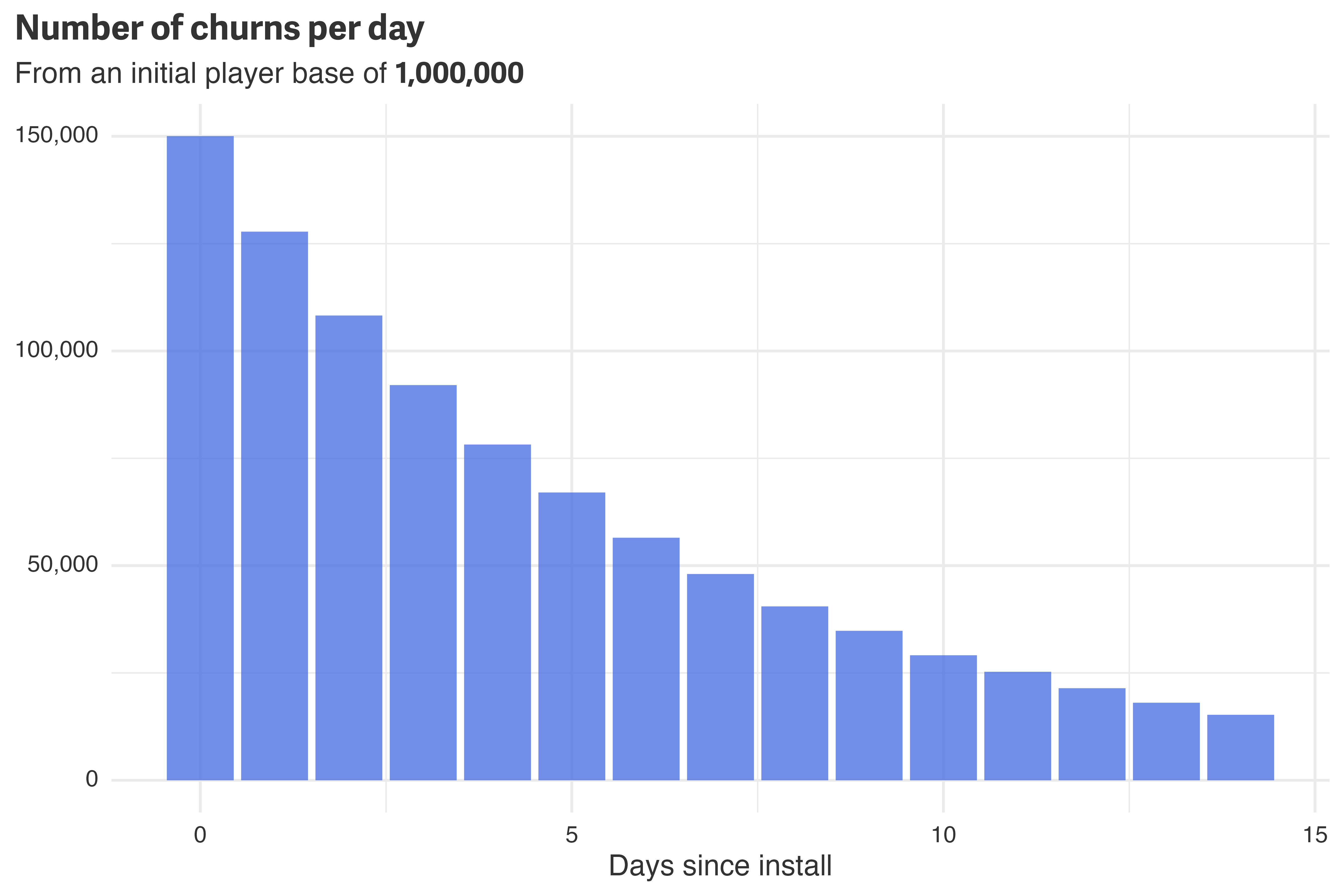

From this data, we might model the churn date, \(T\) as a random draw from an exponential distribution characterized by a rate, \(\lambda\).

\[ T \sim \text{Exponential}(\lambda) \]

There is, however, a slight problem: not all players have churned yet! Of the million initial players, there are still 87,470 players active as of day 15. For these players, we won’t know how many churned on day 15 until we see data for day 16 (hence, there is no daily churn data for day 15 in the chart above). The players in the churn plot are uncensored — we’ve observed their churn date.⁷ To include censored data in the model, we need to dip our toes into a bit of calculus.

⁷ Were this real data, you could strongly argue that all players have censored data. Just because a player isn’t active today doesn’t mean they won’t be active down the line. I’ve simulated the data as explicitly uncensored, so we’re just gonna roll with it for now.

For the remaining active players, we don’t know what their churn date, \(T\), will be. We do know, however, their most recent day of activity, \(t\). Given this, we know that \(T\) must be at least \(t\). From a modeling perspective, we want to know \(\Pr(T \geq t)\). Given an exponential distribution, this corresponds to the shaded area under the probability density function:

Code

tibble(x = 0:30) %>%
  mutate(y = dexp(x, -log(1 - churn_rate)),
         lower = if_else(x < 15, NA, 0),
         upper = if_else(x < 15, NA, y)) %>%
  ggplot(aes(x = x,
             y = y,
             ymin = lower,
             ymax = upper)) +
  geom_vline(xintercept = 15,
             linetype = "dashed",
             color = "gray60") + 
  geom_ribbon(alpha = 0.5,
              fill = "royalblue") + 
  geom_line() +
  scale_y_percent() + 
  theme_rieke() +
  labs(title = "**Probability density of an exponential distribution**",
       subtitle = glue::glue("With a rate of **\u03bb = ",
                             scales::label_number(accuracy = 0.01)(-log(1 - churn_rate)),
                             "**"),
       x = NULL,
       y = NULL)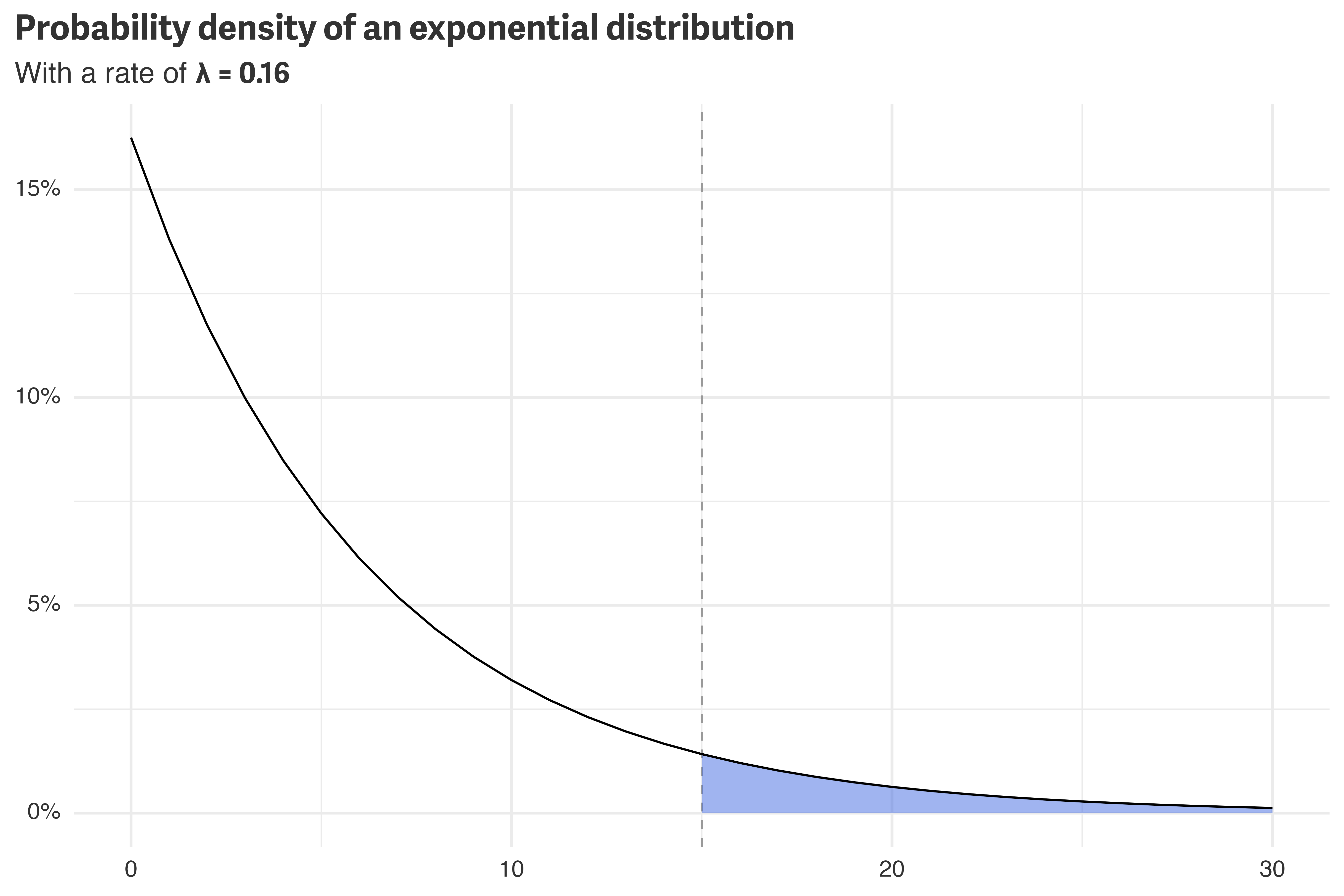

The area under the curve can be evaluated as the integral from \(t\) to \(\infty\). With this, we can add the censored data into the model. For math-y reasons,⁸ \(\lambda\) is connect-able to \(R\) with \(\lambda = -\log(1-R)\).

⁸ The average of an exponential distribution is \(1/\lambda\), so we can just take the inverse of the empirically derived average above.

\[ \begin{align*} T_\text{uncensored} &\sim \text{Exponential}(\lambda) \\ t_\text{censored} &\sim \int_t^\infty \text{Exponential}(\lambda) \\ \lambda &= -\log(1 - R) \\ R &\sim \text{Beta}(1, 1) \end{align*} \]

Code

data {
  // uncensored data
  int<lower=0> N_uncensored;
  vector<lower=0>[N_uncensored] K_uncensored;
  vector<lower=0>[N_uncensored] T_uncensored;
  
  // censored data
  int<lower=0> N_censored;
  vector<lower=0>[N_censored] K_censored;
  vector<lower=0>[N_censored] t_censored;
}
parameters {
  real<lower=0, upper=1> churn_rate;
}
transformed parameters {
  real<lower=0> lambda = -log(1 - churn_rate);
}
model {
  // priors
  target += beta_lpdf(churn_rate | 1, 1);
  
  // likelihood
  target += K_uncensored * exponential_lpdf(T_uncensored | lambda);
  target += K_censored * exponential_lccdf(t_censored | lambda);
}
generated quantities {
  real average_lifetime = inv(lambda);
}

Fitting this model, however, doesn’t recover the simulated parameters as expected! The churn rate is underestimated and the average lifetime is overestimated.⁹

⁹ Stan also complains about NaNS popping up in the calculation of diagnostics.

Code

churn_data <- 
  player_data %>%
  mutate(churned = players - lead(players)) %>%
  drop_na()

censored_data <-
  list(
    N_uncensored = nrow(churn_data),
    K_uncensored = churn_data$churned,
    T_uncensored = churn_data$day,
    N_censored = 1,
    K_censored = n_players - sum(churn_data$churned),
    t_censored = max(player_data$day)
  )

# compile, fit, & display output
censored_model <-
  cmdstan_model("censored_churn.stan")

censored_fit <-
  censored_model$sample(
    data = censored_data,
    iter_warmup = 1000,
    iter_sampling = 1000,
    chains = 4,
    parallel_chains = 4,
    seed = 876
  )

censored_fit$summary() %>%
  filter(variable %in% c("churn_rate", "average_lifetime")) %>%
  select(variable, median, q5, q95) %>%
  knitr::kable()

variable	median	q5	q95
churn_rate	0.131446	0.131394	0.131501
average_lifetime	7.095930	7.092770	7.098970

The problem is due to discrete time. There are about 150,000 players who churn within the first day. Because churn is recorded in discrete days, however, their churn time is recorded as \(T=0\).¹⁰ An exponential distribution changes most rapidly near 0, so not accounting for discrete time steps in the model loses a lot of information.

¹⁰ This problem still occurs if a churn day is redefined to the “first-missed” day (i.e., all churns at \(T=0\) become \(T=1\)). The probelem has to do with discrete time in general.

Model 3: Discrete Censored Regression

In the simulated data, any player who isn’t active by day 1 is counted as churned on day 0. One way to think about this is that any intra-day churns get rounded down in the dataset. For example, \(T=0.7\) and \(T=10.3\) appear as \(T=0\) and \(T=10\) in the dataset, respectively. To mimic this, the model needs to estimate the probability of falling into the range between \(T\) and \(T+1\), rather than just the probability of observing \(T\).

Code

tibble(x = 0:30) %>%
  mutate(y = dexp(x, -log(1 - churn_rate)),
         t0 = if_else(x %in% 0:1, y, NA),
         t10 = if_else(x %in% 10:11, y, NA)) %>%
  ggplot(aes(x = x, 
             y = y)) + 
  geom_ribbon(aes(ymin = 0,
                  ymax = t0),
              fill = "royalblue",
              alpha = 0.75) + 
  geom_ribbon(aes(ymin = 0,
                  ymax = t10),
              fill = "orange",
              alpha = 0.75) + 
  geom_line() +
  scale_y_percent() + 
  theme_rieke() +
  labs(title = "**Probability density of an exponential distribution**",
       subtitle = glue::glue("Probability of falling in **",
                             color_text("(0, 1)", "royalblue"),
                             "** and **",
                             color_text("(10, 11)", "orange"),
                             "**"),
       x = NULL,
       y = NULL)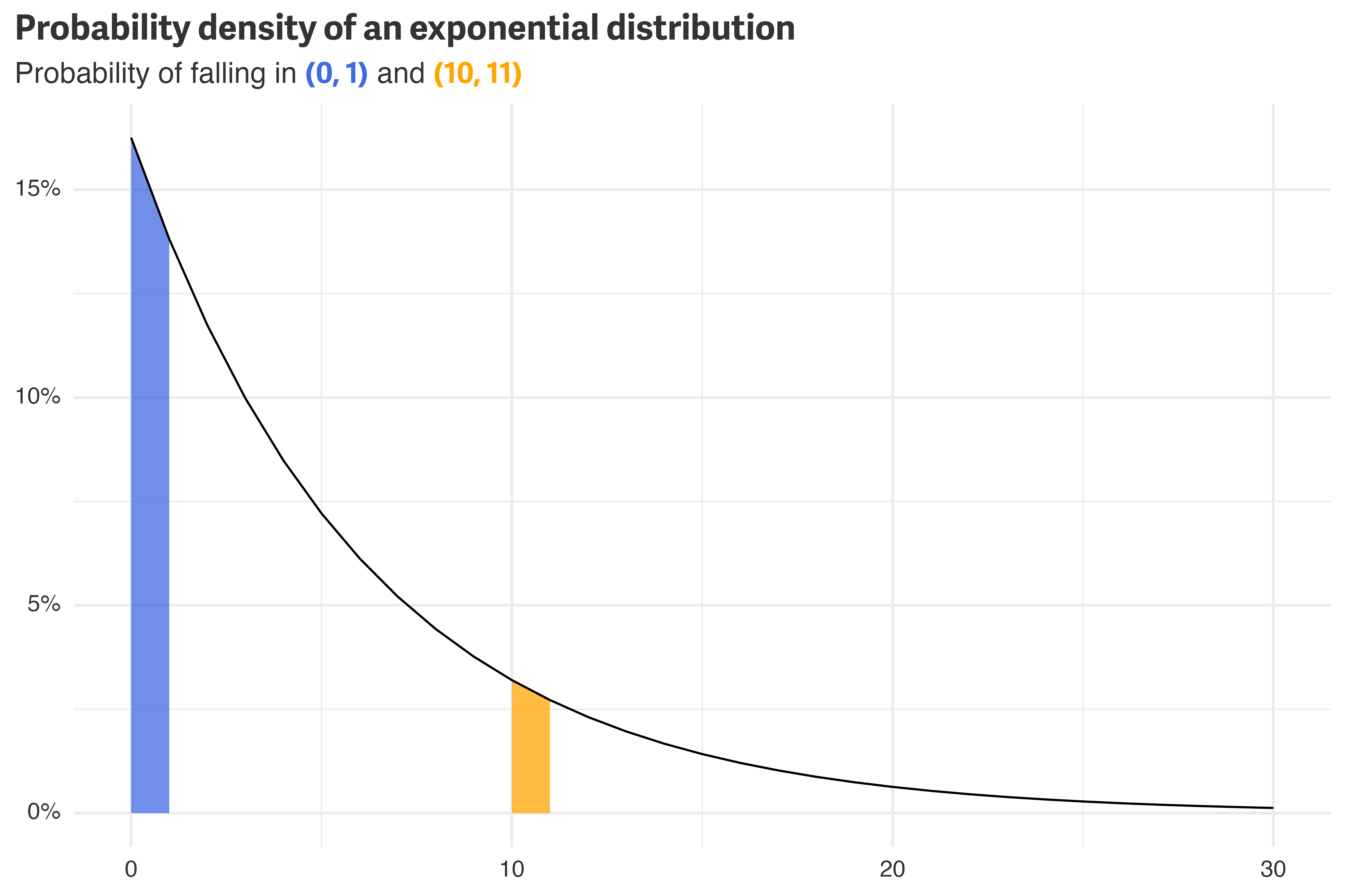

Mathematically, observing a churn at \(T\) can be expressed as the integral of the distribution between \(T\) and \(T+1\).

\[ T_\text{uncensored} \sim \int_T^{T+1} \text{Exponential}(\lambda) \]

Since the probability of observing a censored data point, \(t\), is already estimated with an integral from \(t\) to \(\infty\), there’s no additional changes needed to convert to discrete time. A discrete-time censored model can then be expressed as:

\[ \begin{align*} T_\text{uncensored} &\sim \int_T^{T+1} \text{Exponential}(\lambda) \\ t_\text{censored} &\sim \int_t^\infty \text{Exponential}(\lambda) \\ \lambda &= -\log(1 - R) \\ R &\sim \text{Beta}(1, 1) \end{align*} \]

Code

data {
  // uncensored data
  int<lower=0> N_uncensored;
  vector<lower=0>[N_uncensored] K_uncensored;
  vector<lower=0>[N_uncensored] T_uncensored;
  
  // censored data
  int<lower=0> N_censored;
  vector<lower=0>[N_censored] K_censored;
  vector<lower=0>[N_censored] t_censored;
}
parameters {
  real<lower=0, upper=1> churn_rate;
}
transformed parameters {
  real<lower=0> lambda = -log(1 - churn_rate);
}
model {
  // priors
  target += beta_lpdf(churn_rate | 1, 1);
  
  // likelihood
  for (n in 1:N_uncensored) {
    if (T_uncensored[n] == 0) {
      target += K_uncensored[n] * exponential_lcdf(T_uncensored[n] + 1 | lambda);
    } else {
      real prob = exponential_cdf(T_uncensored[n] + 1 | lambda) - exponential_cdf(T_uncensored[n] | lambda);
      target += K_uncensored[n] * log(prob);
    }
  }
  target += K_censored * exponential_lccdf(t_censored | lambda);
}
generated quantities {
  real average_lifetime = inv(lambda);
}

Fitting the discrete model recovers the expected parameters from simulation: a 15% churn rate and an average lifetime of about 6.2 days.

Code

# same data passed to the new model
discrete_censored_data <- censored_data

# compile, fit, & display output
discrete_censored_model <-
  cmdstan_model("discrete_censored_churn.stan")

discrete_censored_fit <-
  discrete_censored_model$sample(
    data = discrete_censored_data,
    iter_warmup = 1000,
    iter_sampling = 1000,
    chains = 4,
    step_size = 0.002,
    parallel_chains = 4,
    seed = 876
  )

discrete_censored_fit$summary() %>%
  filter(variable %in% c("churn_rate", "average_lifetime")) %>%
  select(variable, median, q5, q95) %>%
  knitr::kable()

variable	median	q5	q95
churn_rate	0.15005	0.149814	0.150285
average_lifetime	6.15089	6.140479	6.161441

Closing thoughts

Censored models are a useful set of tools for working with customer churn data. Data in the wild, however, may not necessarily live up to the assumptions that most out-of-the-box censored regression models make: that events occur in continuous time after \(t=0\). The discrete censored model presented above bridges the gap between model assumptions and the reality of data collection. By modeling events that are recorded in discrete time as the probability of occurring between two continuous time points, the discrete censored model allows for a censored model to be fit to data aggregated into discrete time steps.

In the particular examples above, the models assumed a constant churn rate. This was an appropriate assumption in this case, but may not always be. Alternatives to the exponential distribution, such as the Weibull or gamma can be used to model time-varying churn, or time itself could be included as a model component in estimating a distribution’s parameter. Further, in the above example, all players join the game on the exact same day. In reality, players (or, in general, customers), will have different real-world times that correspond to \(t=0\), and datasets contain more than one censored datapoint.

Regardless of model complexity, average customer lifetime can be derived from a distribution of churn data and a discrete censored model offers a way to estimate the underlying churn distribution while respecting the format that the data was aggregated.

Citation

BibTeX citation:

@online{rieke2023,
  author = {Rieke, Mark},
  title = {Churn, Baby, Churn},
  date = {2023-11-24},
  url = {https://www.thedatadiary.net/posts/2023-11-24-churn-modeling},
  langid = {en}
}

For attribution, please cite this work as:

Rieke, Mark. 2023. “Churn, Baby, Churn.” November 24, 2023. https://www.thedatadiary.net/posts/2023-11-24-churn-modeling.