Roughly 500 days from now (485, if you really want to be picky), Americans will once again line up at polling locations to cast their vote for the next president. If current Republican primary polling holds, the contest will be a rematch of the 2020 election between Biden and Trump, and early head-to-head polling suggests a tight race. Presidential polling this far out, however, isn’t useful for predicting the outcome of the election. In the absence of predictive polling, much (online) ink has been spilled in speculation of Biden’s odds of re-election. Folks place Biden’s chances of winning another term somewhere roughly between a guaranteed loss and a guaranteed victory. In this post, I’ll introduce a simple model that can be used as a prior for the 2024 election and explain why you can (mostly) avoid thinking about it until next year.
A Time for Change
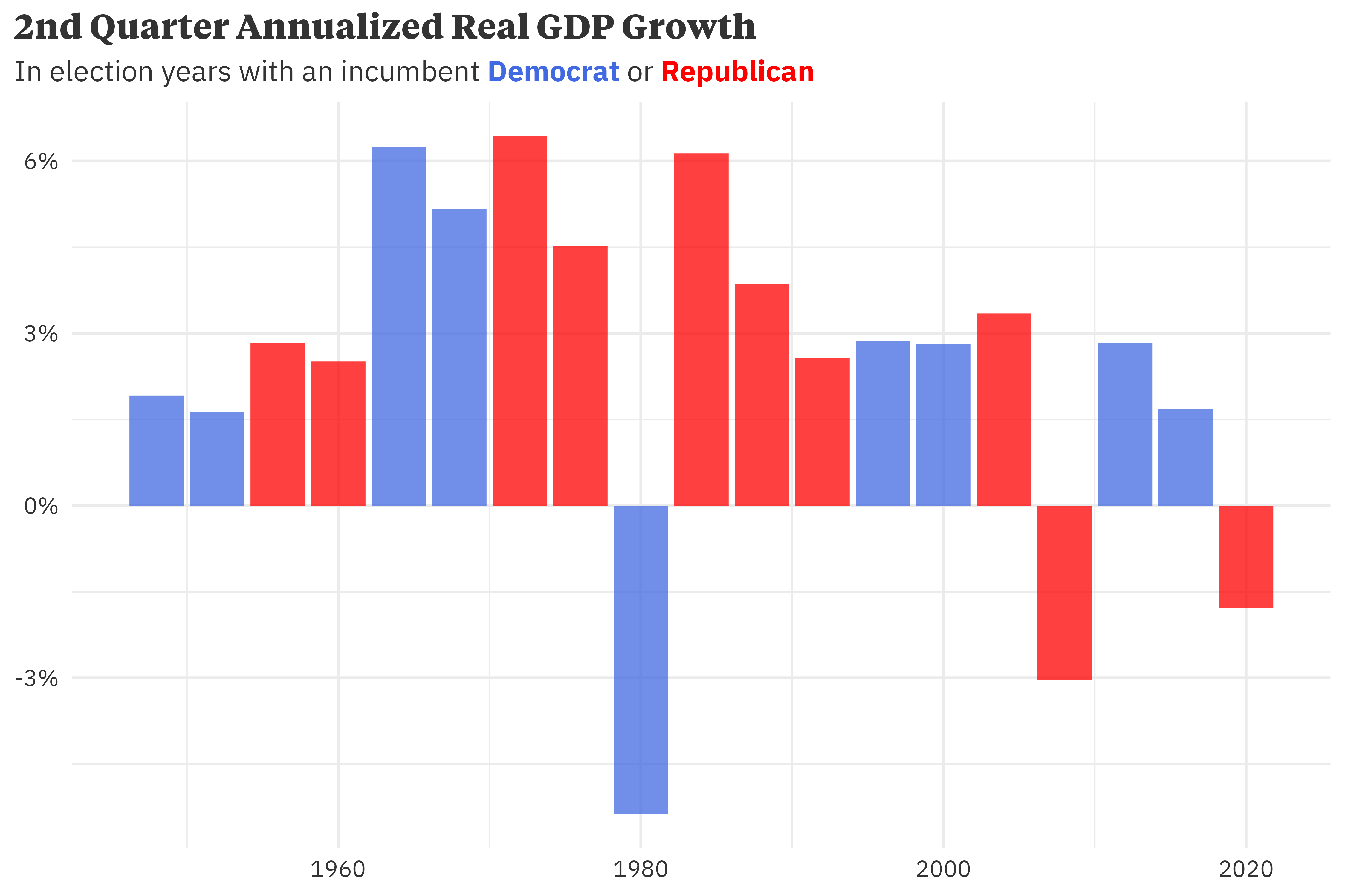
In 1992, challenger Bill Clinton foiled George H.W. Bush’s chance at a second presidential term. His successful campaign was based, in part, on the simple, resounding message of “It’s the economy, stupid.”. Although Bush didn’t preside over negative GDP growth like Jimmy Carter, his term saw middling economic growth relative to his republican predecessors, and the Clinton campaign was able use the early 1990s recession as an attack against a second Bush term.
Bush’s downfall wasn’t, however, solely the result of America’s economic performance. He was also a deeply unpopular president — per 538’s presidential approval tracker, he entered election day with a -22.4% net approval. Although the two variables are likely intertwined, accounting for only one or the other doesn’t provide a clear picture of what the results of an election will be.
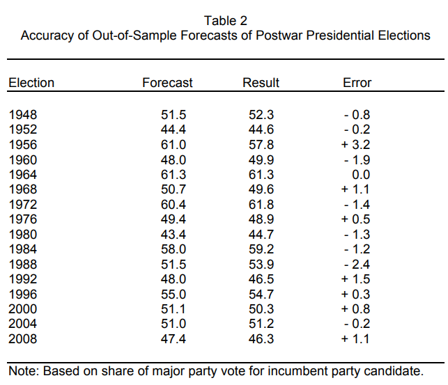
In 1988, political scientist Alan Abramovitz introduced a simple model, dubbed the Time for Change Model, to predict the incumbent party’s two-party voteshare in presidential elections. Under the assumption that a presidential election is a referendum on the incumbent party, Abramovitz’ model is able to fairly accurately project the results of the election based on three variables: the incumbent’s net approval rating, the change in real GDP in the second quarter of the election year, and first term incumbency advantage:
\[ \begin{align*} V_{\text{incumbent}} &= \alpha + \beta_{\text{approve}}A + \beta_{\text{GDP}}G + \beta_{\text{incumbent}}I \end{align*} \]
A change to the Time for Change
Abramovitz’ model provides a clean picture of the expected outcome of the national two-party vote. In presidential elections, however, winning the popular vote doesn’t guarantee a win to office. Candidates must win enough strategic state races to ensure they receive at least 270 electoral college votes. Further, Abramovitz’ model only estimates the two-party vote and doesn’t include estimations for third-party candidates. In American elections, third parties can (generally) be excluded from a model that still provides accurate forecasts. Including third parties, however, gets us closer to the actual process that generates election results.
To address both these concerns, I introduce a two-stage prior model. Firstly, I build on Abramovitz’ work and model the national voteshare of the incumbent party, non-incumbent party, and any third parties, using incumbent net approval, real GDP growth, and incumbency advantage. I also include a term for the presence of a major third party on the ballot. Secondly, the state results are estimated using the 3 party partisan lean (3-PVI). With the state-level results, I can simply add up the electoral college votes each candidate wins to project the winner.
The national model
We can model the national voteshare with a Dirichlet distribution. The Dirichlet distribution in this case is useful as the results of the distribution always sum to 1. Given this, the voteshare, \(V\), of the incumbent party, non-incumbent party, and other parties is estimated with a probability vector, \(P\).
\[ \begin{align*} V & \sim \text{Dirichlet}(P) \\ V & = \langle v_{\text{incumbent}},\ v_{\text{non-incumbent}},\ v_{\text{other}}\rangle \\ P & = \langle p_{\text{incumbent}},\ p_{\text{non-incumbent}},\ p_{\text{other}}\rangle \\ \end{align*} \]
\(P\) can be mapped to a series of linear models, \(\phi\), with the \(\text{softmax}\) function, which converts a group of values on the real scale to an interval between (0, 1). It also ensures that the resulting output sums to 1 (which is needed for probability distributions!).
\[ P = \text{softmax}(\langle \phi_{\text{incumbent}},\ \phi_{\text{non-incumbent}},\ \phi_{\text{other}}\rangle) \]
Each \(\phi\) term is modeled separately. To ensure the model is identifiable, \(\phi_{\text{other}}\) is defined in relation to \(\phi_{\text{incumbent}}\) and \(\phi_{\text{non-incumbent}}\) using the sum-to-zero constraint.
\[ \begin{align*} \phi_{\text{incumbent}} & = \alpha_1 + \beta_{\text{approve},1}A + \beta_{\text{GDP},1}G + \beta_{\text{incumbent},1}I + \beta_{\text{third-party},1}T \\ \phi_{\text{non-incumbent}} & = \alpha_2 + \beta_{\text{approve},2}A + \beta_{\text{GDP},2}G + \beta_{\text{incumbent},2}I + \beta_{\text{third-party},2}T \\ \phi_{\text{other}} & = - (\phi_{\text{incumbent}} + \phi_{\text{non-incumbent}}) \end{align*} \]
Here, \(A\), \(G\), and \(I\) are equivalent to their Time for Change counterparts. \(T\) indicates the presence of a third party in the national race, defined as any individual third-party candidate polling above 5%.
To generate a distribution of results, I implemented the model in Stan and set informative priors over the \(\alpha\) and \(\beta\) parameters — you can view the full model code here.
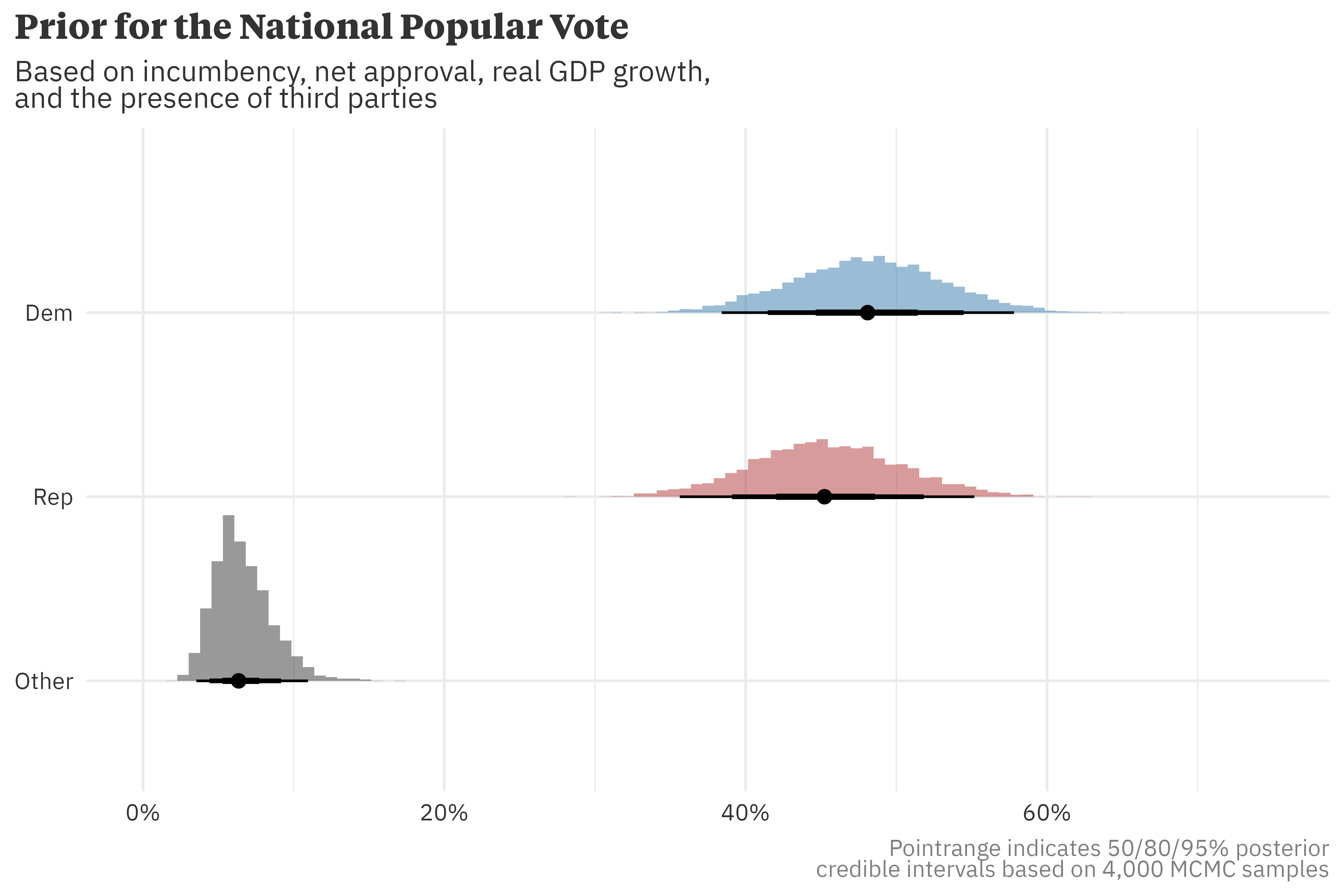
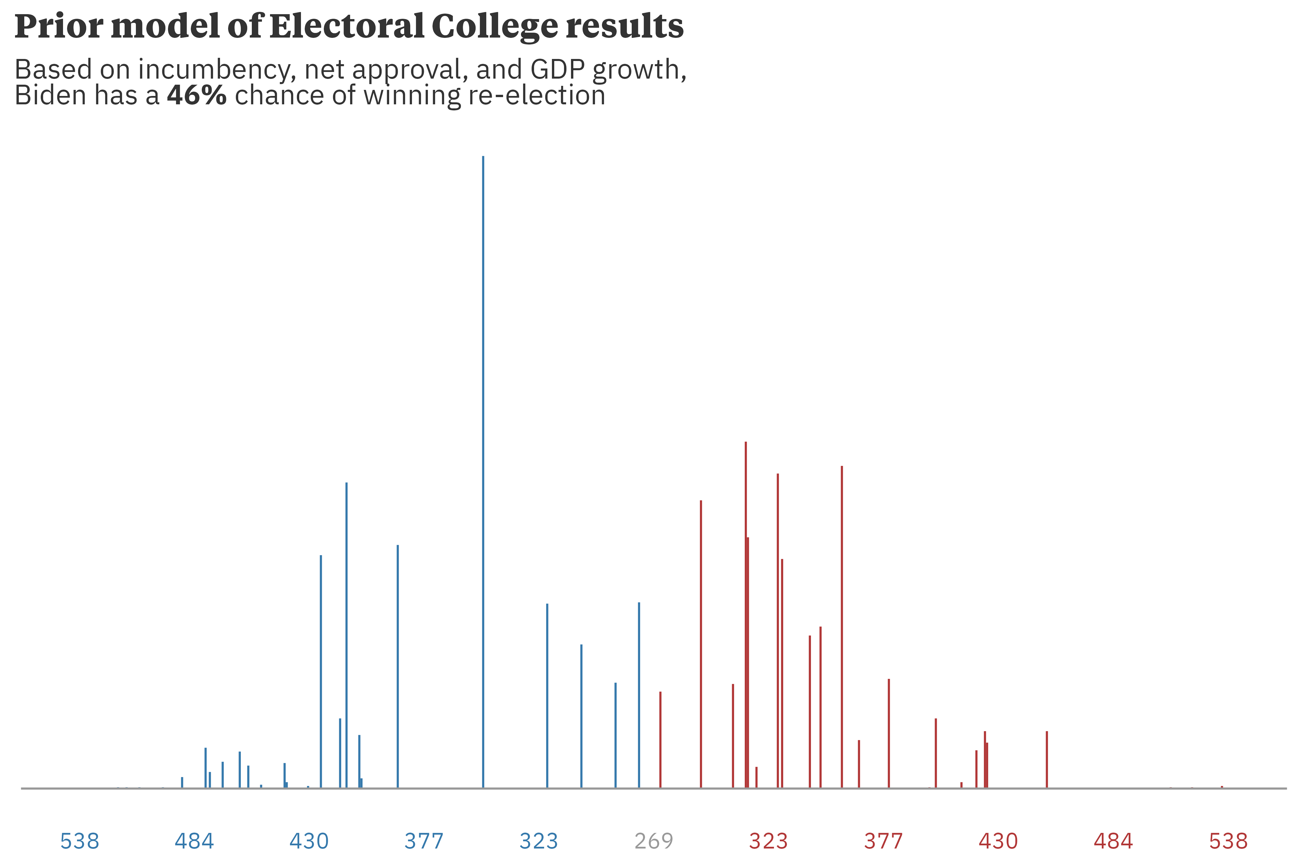
Based on his current net approval, -13.6%, and the most recent quarterly GDP data, which puts real annualized growth at 0.8%, Biden is expected to win the national popular vote, though there is a lot of uncertainty around this estimate. As mentioned above, however, the national result doesn’t determine the winner, and we must turn to the statewide results.
State-level results and the Electoral College
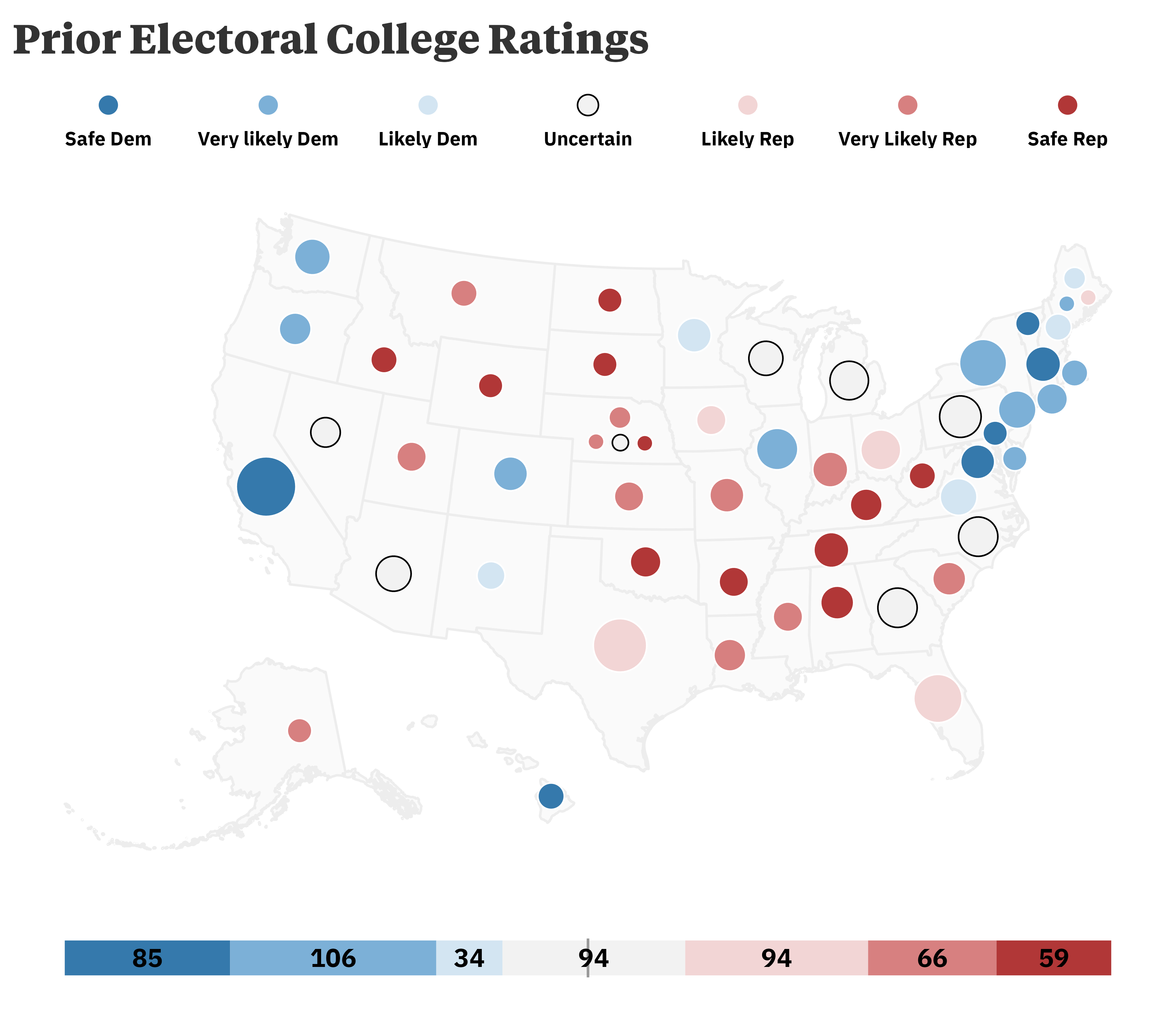
A useful way to think about states is in terms of partisan lean relative to the nation as a whole. For example, in a “blue wave” year, there will still be states that vote solidly for republican candidates, though we’d expect their margin of victory to shift with the nation. To estimate state-level results, I simply added the partisan lean of each state (measured by 3PVI) to the national results. Because the Stan model produced a distribution of national results, adding partisan lean also produces a distribution of state results. There were no simulations in which a third party candidate won any state, so Biden’s probability of winning any given state (expressed as a percentage in the chart below) is simply the proportion of simulations in which he beats his republican challenger.
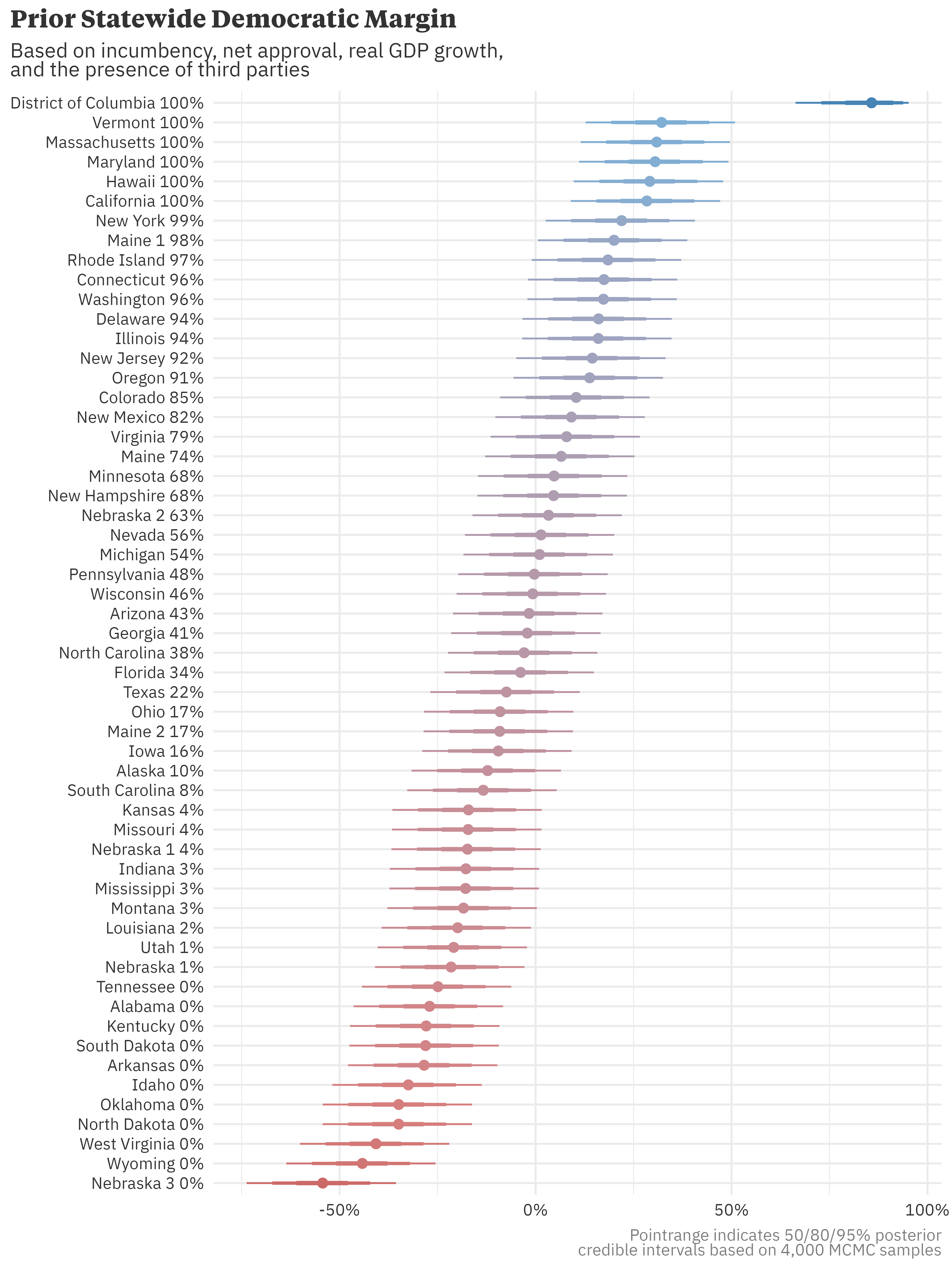
Taking Biden’s probability of winning each state and multiplying it by the number of electors that state provides the expected number of democratic electors. This puts Biden’s expected number of electors won at 279, just above the 270 vote threshold to secure the presidency. This method yields the average outcome but in reality, electoral college votes aren’t “averaged out” — each state allocates all of its votes to the winner. A better method is to take the total number of simulations in which Biden wins enough states to earn at least 270 votes in the electoral college. Doing so shows that, based on this prior model, he has about a 46% chance of winning re-election.
When to update your priors
The output from this model is, explicitly, to be used as a prior. Barring drastic economic change or presidential scandal, I don’t expect this model’s output to shift significantly ahead of June 2024, when we expect polling to start becoming more informative. When that time comes, outlets will release forecasts, and we can start to incorporate more information to update the prior generated from this model. Until then, we can summarize our beliefs with two statements: there is a lot of uncertainty in the outcome of the 2024 election and this uncertainty points to a toss-up between Biden and his eventual challenger.
Programming notes
Although my recommendation is to not spend too much time thinking about the 2024 election until next summer, I’ve recently been spending too much time thinking about the 2024 election. I’m planning on releasing a presidential forecast, which is going to require quite a bit of work (on both the statistics and software engineering spectrum). The model outputs will be released on this site, but you can follow along the development on GitHub. The code for the model in this article along with the code to generate all the plots are also stored in the repository.
Citation
@online{rieke2023,
  author = {Rieke, Mark},
  title = {A {Change} to the {Time} for {Change}},
  date = {2023-07-09},
  url = {https://www.thedatadiary.net/posts/2023-07-09-change-time-for-change/},
  langid = {en}
}