Su-fish-iency

library(tidyverse)
library(cmdstanr)
library(ggdist)
library(riekelib)

# Setup a color palette to be used for groups A/B
pal <- NatParksPalettes::NatParksPalettes$Acadia[[1]][c(2,8)]

Alright, it seems as though I’ve accidentally stumbled my way into a series all about sufficiency. This post on a stable implementation of the sufficient poisson is the latest in a quest to find sufficient formulations for as many distributions as possible (see, for example, my previous posts on the sufficient gamma and sufficient normal). In this case, however, I actually don’t recommend using the sufficient poisson and instead recommend using the pseudo-sufficient count-of-counts method, which I detail below. That being said, if you do want to implement a stable sufficient poisson in stan, you can use this log-likelihood function.

real sufficient_poisson_lpdf(
  real Xsum,
  real Xsumlgamma1,
  real n,
  real lambda
) {
  return (log(lambda) * Xsum) - (lambda * n) - Xsumlgamma1;
}

Possibly Poisson

As always, I’ll start by simulating 5,000 observations from two groups for a total of 10,000 observations in the dataset that will be used across model comparisons. Here, I simulate poisson observations with means 2 and 10.

set.seed(2026)
poisson_data <-
  tibble(group = c("A", "B"),
         lambda = c(2, 10)) %>%
  mutate(y = map(lambda, ~rpois(5000, .x)))

poisson_data %>%
  unnest(y) %>%
  ggplot(aes(x = y,
             y = group,
             fill = group)) +
  stat_histinterval(slab_alpha = 0.75,
                    breaks = \(x) seq(from = min(x), to = max(x), by = 1)) +
  scale_fill_manual(values = pal) +
  theme_rieke()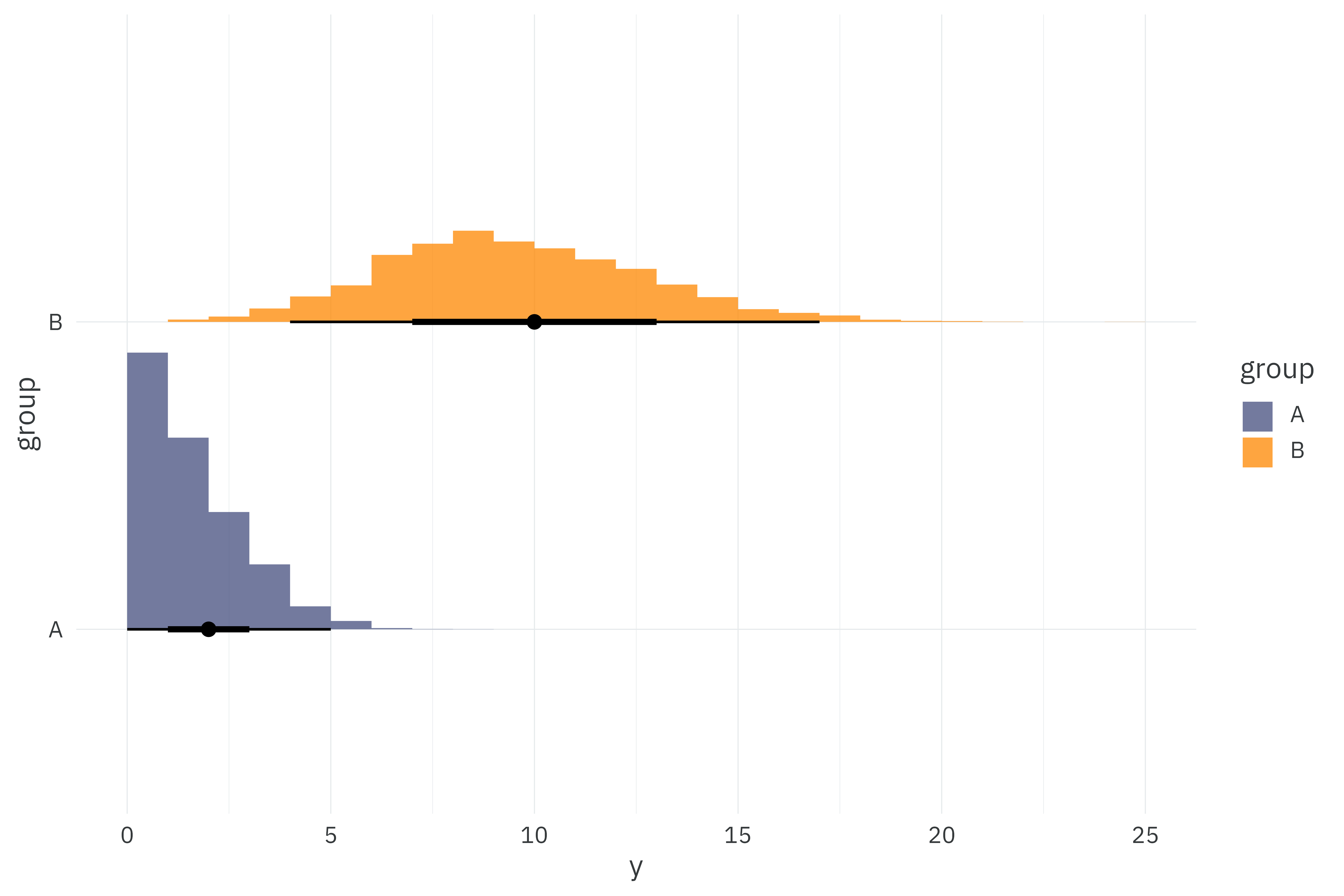

We’ll fit a super-simple poisson likelihood to these observations with a separate mean, \(\lambda\) per group, \(g\).

\[ \begin{align*} y_i &\sim \text{Poisson}(\lambda_g) \\ \lambda_g &\sim \text{Exponential}(1) \end{align*} \]

data {
  // Dimensions
  int<lower=0> N;                          // Number of observations
  int G;                                   // Number of groups

  // Observations
  array[N] int<lower=0> Y;                 // Outcome per observation
  array[N] int<lower=1, upper=G> gid;      // Group membership per observation
  
  // Poisson priors
  real<lower=0> lambda_lambda;
}

parameters {
  vector<lower=0>[G] lambda;
}

model {
  target += exponential_lpdf(lambda | lambda_lambda);
  for (n in 1:N) {
    target += poisson_lpmf(Y[n] | lambda[gid[n]]);
  }
}

individual_model <- cmdstan_model("individual-poisson.stan")

make_individual_data <- function() {

  model_data <- 
    poisson_data %>%
    mutate(gid = rank(group)) %>%
    unnest(y)

  stan_data_individual <-
    list(
      N = nrow(model_data),
      Y = model_data$y,
      G = max(model_data$gid),
      gid = model_data$gid,
      lambda_lambda = 1
    )
    
  return(stan_data_individual)
}

stan_data_individual <- make_individual_data()

start_time <- Sys.time()
individual_fit <-
  individual_model$sample(
    data = stan_data_individual,
    seed = 1234,
    iter_warmup = 1000,
    iter_sampling = 1000,
    chains = 10,
    parallel_chains = 10
  )
run_time_individual <- as.numeric(Sys.time() - start_time)

plot_posterior <- function(fit) {
  
  # Get the true parameters used in simulation
  truth <- 
    poisson_data %>%
    select(group, lambda) %>%
    pivot_longer(-group,
                 names_to = "parameter",
                 values_to = "draw") %>%
    mutate(parameter = "\u03bb")
  
  fit$draws("lambda", format = "df") %>%
    as_tibble() %>%
    select(starts_with("lambda")) %>%
    pivot_longer(everything(),
                 names_to = "parameter",
                 values_to = "draw") %>%
    nest(data = -parameter) %>%
    separate(parameter, c("parameter", "group"), "\\[") %>%
    mutate(group = str_remove(group, "\\]"),
           group = if_else(group == "1", "A", "B")) %>%
    mutate(parameter = "\u03bb") %>%
    unnest(data) %>%
    ggplot(aes(x = draw,
               y = parameter,
               fill = group)) +
    stat_histinterval(breaks = 60,
                      slab_alpha = 0.75) +
    geom_point(data = truth,
               color = "red") +
    scale_fill_manual(values = pal) +
    theme_rieke()
  
}

plot_posterior(individual_fit) +
  labs(title = "**Fit against individual observations**",
       subtitle = "Can be used as a baseline for evaluating the sufficient formulation",
       x = NULL,
       y = NULL) +
  expand_limits(x = 0)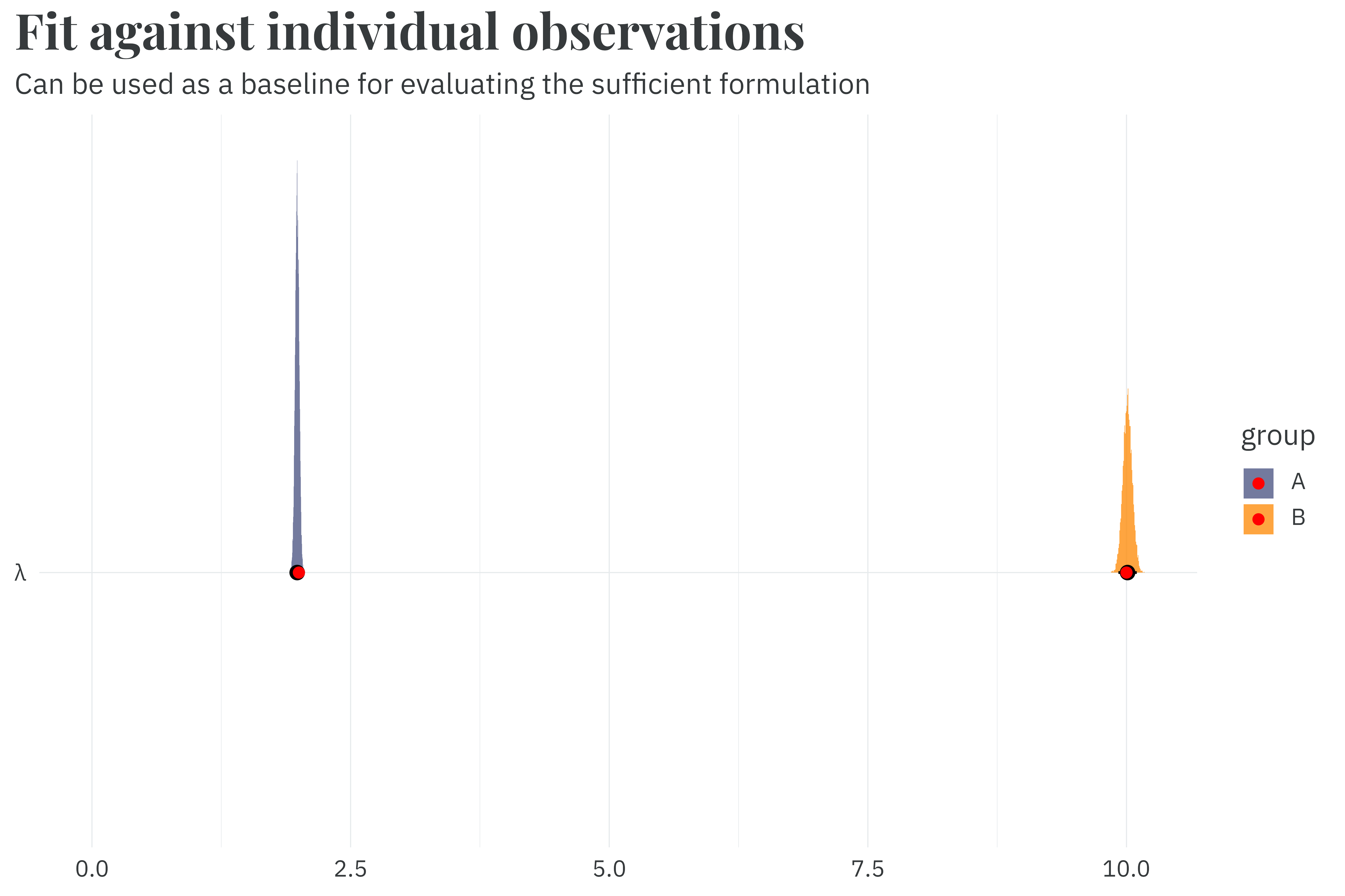

Fitting against individual observations recovers the parameters used during simulation in 3.3 seconds. This is good, but we can potentially improve by being a bit smarter with our dataset.

Counts of counts

During fitting, the model takes each observation in the dataset, finds the probability of having observed that value from a poisson distribution with mean \(\lambda\), and adds the log of that probability to a running total (aka, the target density).¹ Because poisson-distributed values are discrete, however, there’s bound to be a lot of repeated observations in our dataset. We can reduce the computational overhead for our model by just multiplying the log-probability for each observation, \(y\), by the number of times it appears in the dataset, rather than adding each individual log-probability.

¹ Just let me anthropomorphize the model, it’s fine.

So in an example dataset with three observations \(y=\{2,3,3\}\), we can reduce the number of log-probability calculations the model needs to make by exploiting the fact that \(3\) is repeated and passing in the number of times it’s repeated as data.

\[ \begin{align*} \log(\Pr(y \mid \lambda)) &= \log(\Pr(2 \mid \lambda)) + \log(\Pr(3 \mid \lambda)) + \log(\Pr(3 \mid \lambda)) \\ &= \log(\Pr(2 \mid \lambda)) + 2 \times \log(\Pr(3 \mid \lambda)) \end{align*} \]

model_data <- 
  poisson_data %>%
  mutate(gid = rank(group)) %>%
  unnest(y) %>%
  count(group, lambda, y, gid) %>%
  rename(K = n)

new_size <- nrow(model_data)
reduction <- 1 - (new_size/10000)

In this trivial example, we only reduced our effective dataset size by one, since there were only three observations. In our simulated example, however, this reduces the effective dataset size from 10,000 to 33, a 99.7% decrease!

model_data

#> # A tibble: 33 × 5
#>    group lambda     y   gid     K
#>    <chr>  <dbl> <int> <dbl> <int>
#>  1 A          2     0     1   675
#>  2 A          2     1     1  1349
#>  3 A          2     2     1  1402
#>  4 A          2     3     1   858
#>  5 A          2     4     1   475
#>  6 A          2     5     1   168
#>  7 A          2     6     1    61
#>  8 A          2     7     1     9
#>  9 A          2     8     1     2
#> 10 A          2     9     1     1
#> # ℹ 23 more rows

We can modify the model code to take in counts of observations for an increase in speed.

data {
  // Dimensions
  int<lower=0> N;                          // Number of observations
  int G;                                   // Number of groups

  // Observations
  array[N] int<lower=0> Y;                 // Outcome per observation
  array[N] int<lower=1> K;                 // Number of observations per outcome Y
  array[N] int<lower=1, upper=G> gid;      // Group membership per observation
  
  // Poisson priors
  real<lower=0> lambda_lambda;
}

parameters {
  vector<lower=0>[G] lambda;
}

model {
  target += exponential_lpdf(lambda | lambda_lambda);
  for (n in 1:N) {
    target += K[n] * poisson_lpmf(Y[n] | lambda[gid[n]]);
  }
}

count_model <- cmdstan_model("counts-of-poisson.stan")

make_count_data <- function() {
  model_data <- 
    poisson_data %>%
    mutate(gid = rank(group)) %>%
    unnest(y) %>%
    count(group, lambda, y, gid) %>%
    rename(K = n)

  stan_data_count <-
    list(
      N = nrow(model_data),
      Y = model_data$y,
      K = model_data$K,
      G = max(model_data$gid),
      gid = model_data$gid,
      lambda_lambda = 1
    )
  
  return(stan_data_count)
}

stan_data_count <- make_count_data()
start_time <- Sys.time()
count_fit <-
  count_model$sample(
    data = stan_data_count,
    seed = 1234,
    iter_warmup = 1000,
    iter_sampling = 1000,
    chains = 10,
    parallel_chains = 10
  )
run_time_count <- as.numeric(Sys.time() - start_time)

This new model samples in just 0.7 seconds, a 4.8x speedup compared to the fit against individual observations. And it still recovers the same posterior from the original fit.

plot_posterior(count_fit)  +
  labs(title = "**Fit using the count of poisson observations**",
       subtitle = "Recovers the same posterior from the fit to individual observations!",
       x = NULL,
       y = NULL) +
  expand_limits(x = 0)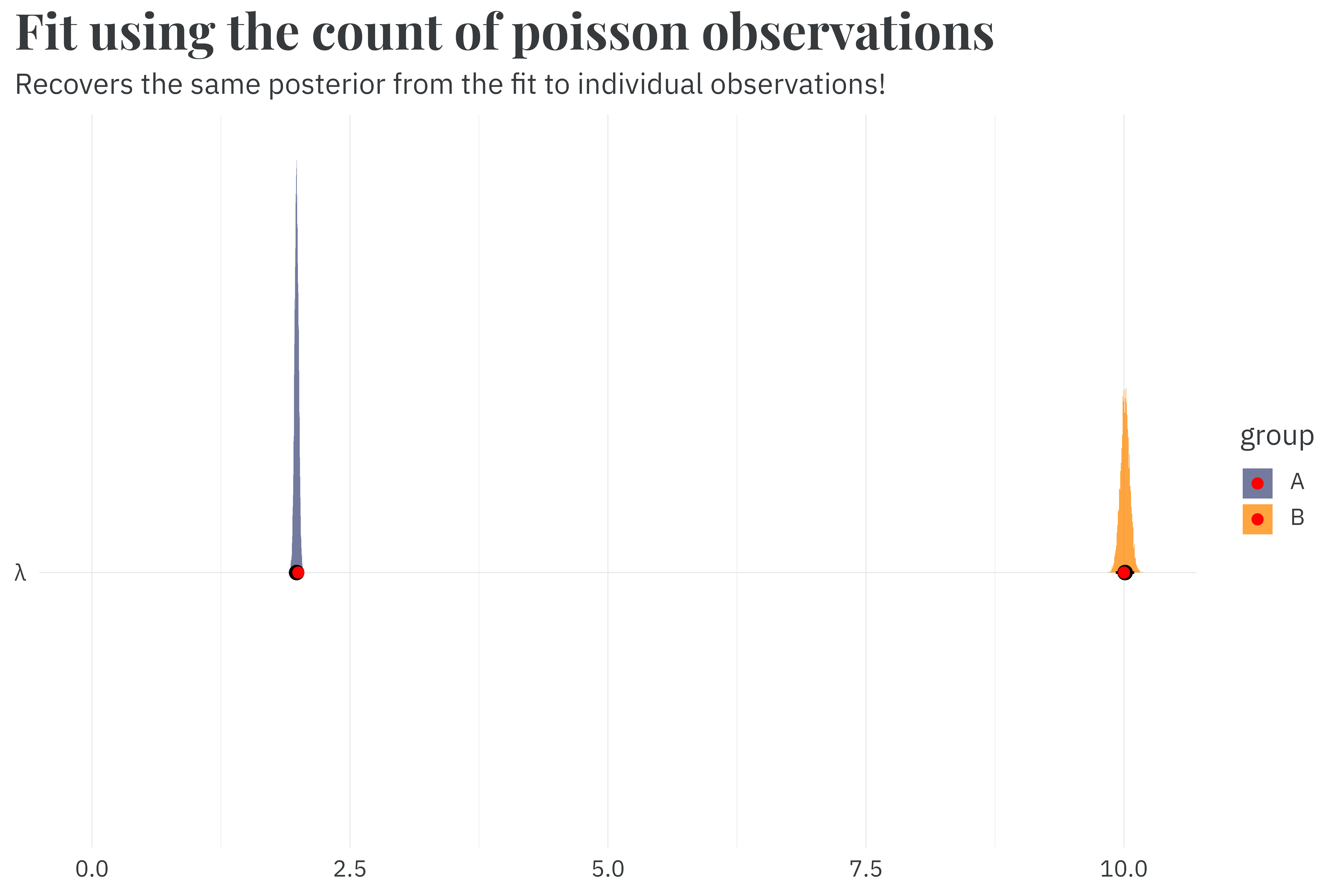

Honestly, this is where you should stop reading. If you need to speed up a poisson model, just use this count-of-counts method. But wading through the density derivation for the sufficient formulation and finding a numerically stable version was fun for me. So if you’re a pedant for math like I am, follow me forward.

Density Derivations

The probability of \(y_i\) given a poisson distribution with mean \(\lambda\) is:

\[ \begin{align*} \Pr(y_i) &= \frac{\lambda^{y_i}e^{-\lambda}}{y_i!} \end{align*} \]

As always, we work on the log scale. Taking the log of the probability yields the following.

\[ \log(\Pr(y_i)) = \log(\lambda) y_i - \lambda - \log(y_i!) \]

Repeatedly incrementing the log-probability over \(y_1, y_2, \dots y_n\) gives the following repeated sum:

\[ \begin{align*} \log(\Pr(y_1, y_2, \dots y_n)) =&\ \log(\lambda)y_1 - \lambda - \log(y_1!) \\ &+ \log(\lambda) y_2 - \lambda - \log(y_2!) \\ &+ \dots \\ &+ \log(\lambda) y_n - \lambda - \log(y_n!) \end{align*} \]

We can summarize this with a sufficient formulation of the log probability given the count and sum of observations in \(y\) as well as the log sum of the factorials of \(y\).

\[ \log(\Pr(y)) = \log(\lambda) \sum y - n\lambda - \sum \log(y!) \]

The un-logged probability density is then:

\[ \Pr\left(\sum y, \sum \log(y!), n \mid \lambda \right) = \frac{\lambda^{\sum y}e^{-\lambda n}}{\prod y!} \]

Sufficient Speedups

With this sufficient formulation, we can collapse our original 10,000 row dataset into just two rows — one per group.

sufficient_model <- cmdstan_model("sufficient-poisson.stan")

model_data <- 
  poisson_data %>%
  mutate(gid = rank(group),
         n = map_int(y, length),
         Ysum = map_dbl(y, sum),
         Ysumlogfact = map_dbl(y, ~sum(log(factorial(.x)))))

model_data

#> # A tibble: 2 × 7
#>   group lambda y               gid     n  Ysum Ysumlogfact
#>   <chr>  <dbl> <list>        <dbl> <int> <dbl>       <dbl>
#> 1 A          2 <int [5,000]>     1  5000  9921       5335.
#> 2 B         10 <int [5,000]>     2  5000 50058      78098.

We can keep the same priors and just swap out our original likelihood function for our new sufficient likelihood.

\[ \begin{align*} \sum y_g, \sum \log(y_g!), n_g &\sim \text{Sufficient-Poisson}(\lambda_g) \\ \lambda_g &\sim \text{Exponential}(1) \end{align*} \]

functions {
  real sufficient_poisson_lpdf(
    real Xsum,
    real Xsumlogfact,
    real n,
    real lambda
  ) {
    return (log(lambda) * Xsum) - (lambda * n) - Xsumlogfact;
  }
}

data {
  // Dimensions
  int<lower=0> N;                          // Number of observations
  int G;                                   // Number of groups

  // Observations
  vector[N] Ysumlogfact;                   // Sum of the log of factorials: sum(log(factorial(Y))) 
  vector[N] Ysum;                          // Sum of observations
  vector[N] n_obs;                         // Number of observations per group
  array[N] int<lower=1, upper=G> gid;      // Group membership per observation
  
  // Poisson priors
  real<lower=0> lambda_lambda;
}

parameters {
  vector<lower=0>[G] lambda;
}

model {
  target += exponential_lpdf(lambda | lambda_lambda);
  for (n in 1:N) {
    target += sufficient_poisson_lpdf(Ysum[n] | Ysumlogfact[n], n_obs[n], lambda[gid[n]]);
  }
}

make_sufficient_data <- function() {
  model_data <- 
    poisson_data %>%
    mutate(gid = rank(group),
           n = map_int(y, length),
           Ysum = map_dbl(y, sum),
           Ysumlogfact = map_dbl(y, ~sum(log(factorial(.x)))))

  stan_data_sufficient <-
    list(
      N = nrow(model_data),
      Ysum = model_data$Ysum,
      Ysumlogfact = model_data$Ysumlogfact,
      n_obs = model_data$n,
      G = max(model_data$gid),
      gid = model_data$gid,
      lambda_lambda = 1
    )

  return(stan_data_sufficient)
}

stan_data_sufficient <- make_sufficient_data()
start_time <- Sys.time()
sufficient_fit <-
  sufficient_model$sample(
    data = stan_data_sufficient,
    seed = 1234,
    iter_warmup = 1000,
    iter_sampling = 1000,
    chains = 10,
    parallel_chains = 10
  )
run_time_sufficient <- as.numeric(Sys.time() - start_time)

Fitting the sufficient formulation only takes 0.7 seconds seconds, a rounding error away from the count-of-count approach and a 5.0x speedup relative to the model fit to individual observations. It recovers the same parameters as expected.

plot_posterior(sufficient_fit)  +
  labs(title = "**Fit using the sufficient poisson**",
       subtitle = "Recovers the same posterior from the fit to individual observations!",
       x = NULL,
       y = NULL) +
  expand_limits(x = 0)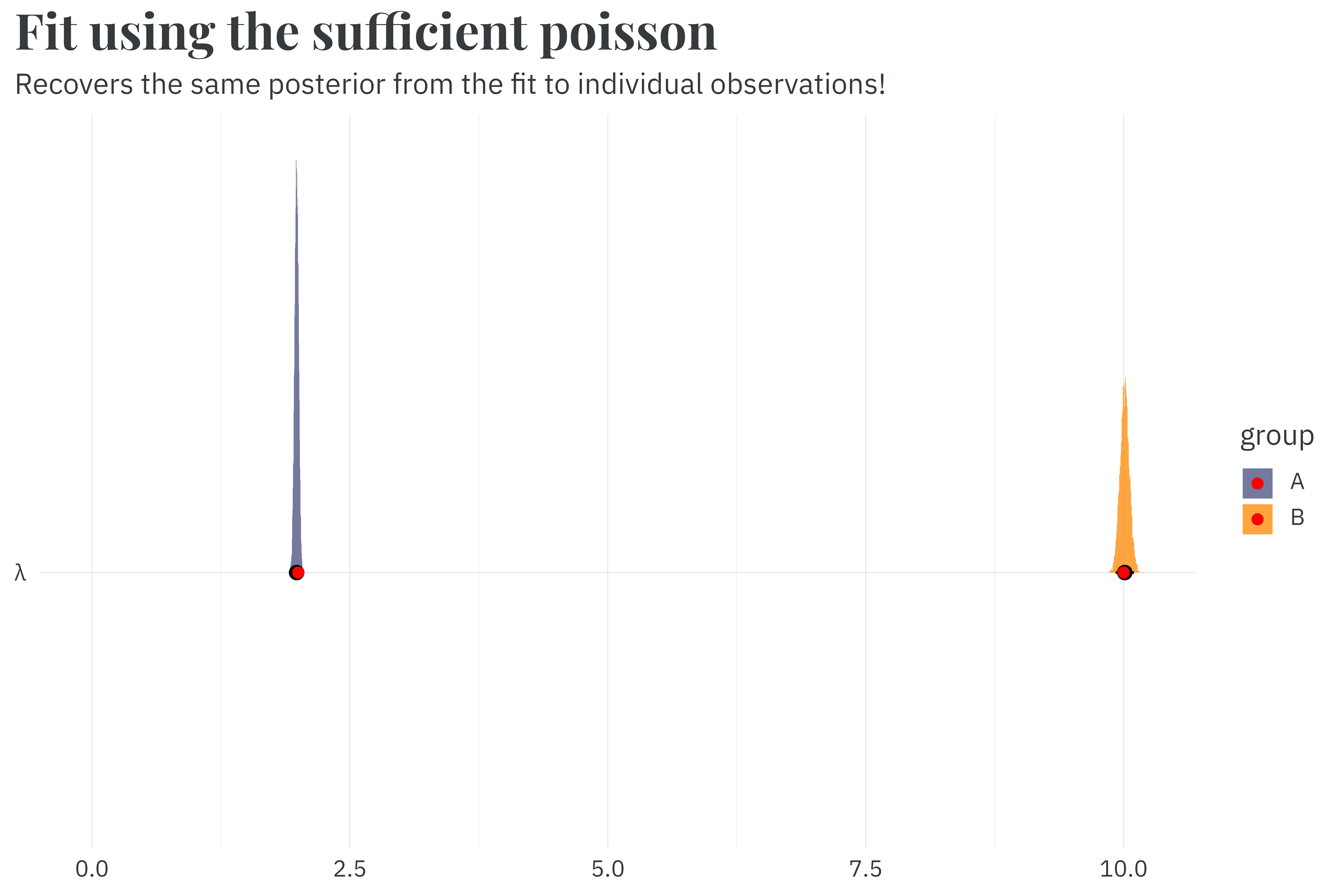

This sufficient implementation works when all observations in \(y\) are relatively small, but it breaks down at large values of \(y\) because the factorial in the denominator just becomes ridiculous to compute directly. Let’s try fitting our models to a new dataset with new group means of 150 and 200.

poisson_data <-
  tibble(group = c("A", "B"),
         lambda = c(200, 150)) %>%
  mutate(y = map(lambda, ~rpois(5000, .x)))

poisson_data %>%
  unnest(y) %>%
  ggplot(aes(x = y,
             y = group,
             fill = group)) +
  stat_histinterval(slab_alpha = 0.75,
                    breaks = \(x) seq(from = min(x), to = max(x), by = 1)) +
  scale_fill_manual(values = pal) +
  theme_rieke()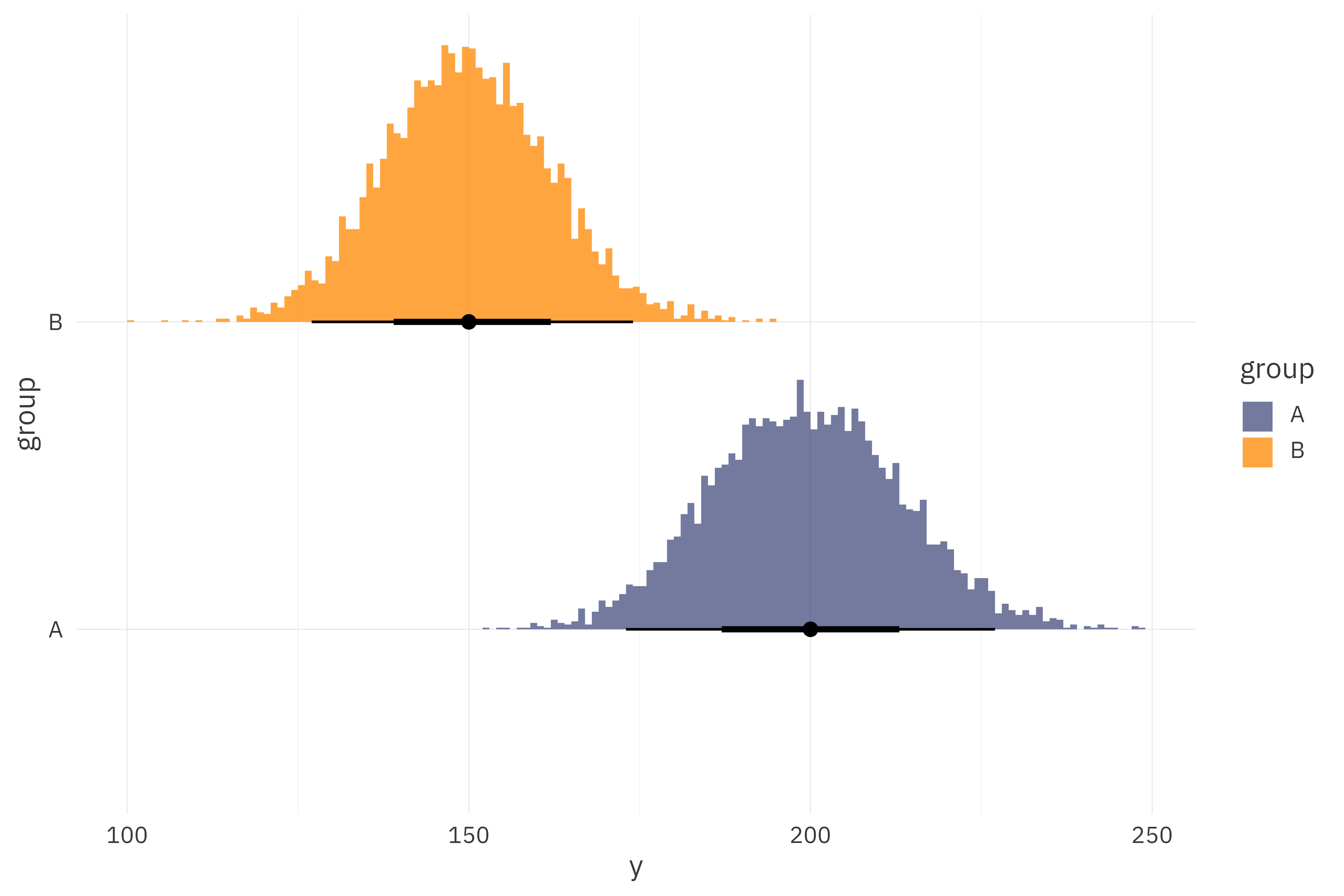

\(200!\) is a 375-digit number — far larger than anything that general-purpose programs can generate. If we try fitting to this new dataset, the individual and count-of-counts models will work just fine. Since R can’t handle a 375-digit number, we’ll end up passing Inf to the sufficient model and fail to sample.

try_sampling <- function(model_name, model, stan_data) {
  tryCatch(
    {
      start_time <- Sys.time()
      model$sample(
        data = stan_data,
        seed = 1234,
        iter_warmup = 1000,
        iter_sampling = 1000,
        chains = 10,
        parallel_chains = 10
      )
      run_time <- as.numeric(Sys.time() - start_time)
      out <- paste("✓", model_name, "model fit in", scales::label_number(accuracy=0.1)(run_time), "seconds")
      return(out)
    },
    warning = function(w) {
      out <- paste("✗", model_name, "model failed to fit!")
      return(out)
    }
  )
}

results <- 
  tibble(model_name = c("individual", "count-of-count", "sufficient"),
         model = c(individual_model, count_model, sufficient_model),
         stan_data = list(make_individual_data(), make_count_data(), make_sufficient_data())) %>%
  mutate(result = pmap_chr(list(model_name, model, stan_data), ~try_sampling(..1, ..2, ..3)))

for (result in results$result) {
  print(result)
}

#> [1] "✓ individual model fit in 2.8 seconds"
#> [1] "✓ count-of-count model fit in 0.7 seconds"
#> [1] "✗ sufficient model failed to fit!"

To avoid crashing into infinity, we can use a numerically stable alternative to the simple factorial by exploiting the fact that \(x! = \Gamma(x+1)\). Thus, our updated log-probability function becomes:

\[ \log(\Pr(y)) = \log(\lambda) \sum y - \lambda n - \sum \log \left(\Gamma(y+1)\right) \]

functions {
  real sufficient_poisson_lpdf(
    real Xsum,
    real Xsumlgamma1,
    real n,
    real lambda
  ) {
    return (log(lambda) * Xsum) - (lambda * n) - Xsumlgamma1;
  }
}

data {
  // Dimensions
  int<lower=0> N;                          // Number of observations
  int G;                                   // Number of groups

  // Observations
  vector[N] Ysumlgamma1;                   // Sum of the log of the Gamma function + 1: sum(lgamma(Y + 1)) 
  vector[N] Ysum;                          // Sum of observations
  vector[N] n_obs;                         // Number of observations per group
  array[N] int<lower=1, upper=G> gid;      // Group membership per observation
  
  // Poisson priors
  real<lower=0> lambda_lambda;
}

parameters {
  vector<lower=0>[G] lambda;
}

model {
  target += exponential_lpdf(lambda | lambda_lambda);
  for (n in 1:N) {
    target += sufficient_poisson_lpdf(Ysum[n] | Ysumlgamma1[n], n_obs[n], lambda[gid[n]]);
  }
}

stable_sufficient_model <- cmdstan_model("stable-sufficient-poisson.stan")

make_stable_sufficient_data <- function() {
  model_data <- 
    poisson_data %>%
    mutate(gid = rank(group),
           n = map_int(y, length),
           Ysum = map_dbl(y, sum),
           Ysumlgamma1 = map_dbl(y, ~sum(lgamma(.x + 1))))
  
  stan_data <-
    list(
      N = nrow(model_data),
      Ysum = model_data$Ysum,
      Ysumlgamma1 = model_data$Ysumlgamma1,
      n_obs = model_data$n,
      G = max(model_data$gid),
      gid = model_data$gid,
      lambda_lambda = 1
    )

  return(stan_data)
}

stable_results <- 
  tibble(model_name = "stable-sufficient",
         model = list(stable_sufficient_model),
         stan_data = list(make_stable_sufficient_data())) %>%
  mutate(result = pmap_chr(list(model_name, model, stan_data), ~try_sampling(..1, ..2, ..3)))

results <-
  results %>%
  bind_rows(stable_results)

for (result in results$result) {
  print(result)
}

#> [1] "✓ individual model fit in 2.8 seconds"
#> [1] "✓ count-of-count model fit in 0.7 seconds"
#> [1] "✗ sufficient model failed to fit!"
#> [1] "✓ stable-sufficient model fit in 0.7 seconds"

The sufficient poisson is really just a mathematical curiosity. You should just use the count-of-counts method — you still get a massive reduction in the dataset size and increase in sampling speed for far less of the mental overhead of the sufficient poisson. If you are going to use a sufficient poisson, make use of the stable variant.